
Introduction
Dry reforming of methane (DRM) utilizes methane (CH4) and carbon dioxide (CO2), the two major sources of greenhouse gas (GHG) emissions and main components of biogas, to produce pure hydrogen (H2) or a mixture of H2 and CO known as syngas. DRM is quite appealing as it reduces the amount of GHGs emissions, valorizes organic waste and produces syngas which can be used as an alternative to fossil fuels.
This application model demonstrates the process of modeling H2 production from dry methane reforming of biogas in a fluidized bed reactor. The simulation exemplifies the usage of compressible isothermal flow setup with volumetric chemistry in Barracuda Virtual Reactor (referred to as Barracuda in rest of this application model post).
Model Definition
The reactor geometry modeled in this application is sourced from the work of Ugarte et. al’ 2017. Figure 1 shows the reactor model geometry, 2.8 cm in diameter and 30 cm in height. 15 g of Ni-based catalyst (5% Ni/Al2O3) is used in the reactor. The temperature of reactor wall is fixed at 873.15 K and the initial catalyst bed height in the reactor is set to 7.3 cm. CH4:CO:Ar at a molar ratio of 4:4:2 are injected from the bottom flow BC at a velocity of 0.0122 m/sec to fluidize bed. The top boundary is defined as a pressure BC at atmospheric pressure.
The Ni-based catalyst particle sizes are between 106-180 microns. WenYu-Ergun drag model is used for capture the interaction between fluids and solid catalyst particles. The material properties of gases and solid particles are a function of temperature in this simulation. All gases are assumed to show ideal gas behavior.
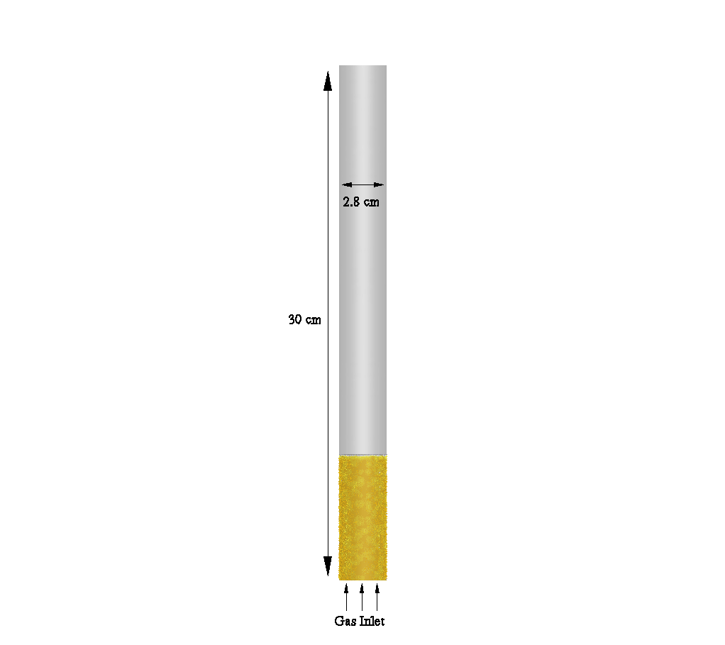
Figure 1: Dry Methane Reforming Simulation Domain.
Reaction Kinetics
Dry reforming of methane can be described using five global reaction steps. These include the main DRM reaction, reverse water gas shift (RWGS) reaction, methane decomposition (MD), steam gasification (SG) and Boudouard reaction (BR)
$$ DRM: CH_4 + CO_2 \iff 2H_2 + 2CO $$
$$ RWGS: CO_2 + H_2 \iff CO + H_2O $$
$$ MD: CH_4 \iff C + 2H_2 $$
$$ SG: C + H_2O \iff CO + H_2 $$
$$ BR: C + CO_2 \iff 2CO $$
The reaction kinetics for the DRM process, taken from Benguerba et.al’ 2015 are shown below,
\begin{align}
R_1 &= \frac{k_{1} K_{CO_2,1} K_{CH_4,1} P_{CH_4} P_{CO_2}}{ \left( 1 + K_{CO_2,1} P_{CO_2} + K_{CH_4,1} P_{CH_4} \right)^2} \left( 1 – \frac{\left( P_{CO} P_{H_2}\right)^2}{K_{P_1} \left( P_{CH_4} P_{CO_2} \right) } \right) \\
R_2 &= \frac{k_{2} K_{CO_2,2} K_{H_2,2} P_{CO_2} P_{H_2}}{ \left( 1 + K_{CO_2,2} P_{CO_2} + K_{H_2,2} P_{H_2} \right)^2} \left( 1 – \frac{\left( P_{CO} P_{H_2O}\right)}{K_{P_2} \left( P_{CO_2} P_{H_2} \right) } \right) \\
R_3 &= \frac{k_{3} K_{CH_4,3} \left( P_{CH_4} – \frac{P_{H_2}^2}{K_{P_3}} \right)}{ \left( 1 + K_{CH_4,3} P_{CH_4} + \frac{1}{K_{H_2,3}} P_{H_2}^{1.5} \right)^2} \\
R_4 &= \frac{ \frac{k_{4}} {K_{H_2O,4}} \left( \frac{P_{H_2O}}{P_{H_2}} – \frac{P_{CO}}{K_{P_4}} \right)}{ \left( 1 + K_{CH_4,4} P_{CH_4} + \frac{1}{K_{H_2O,4}} \frac{P_{H_2O}}{P_{H_2}} + \frac{1}{K_{H_2,4}} P_{H_2}^{1.5} \right)^2} \\
R_5 &= \frac{ \frac{k_{5}} {K_{CO,5} K_{CO_2,5} } \left( \frac{P_{CO_2}}{P_{CO}} – \frac{P_{CO}}{K_{P_5}} \right)}{ \left( 1 + K_{CO,5} P_{CO} + \frac{1}{K_{CO,5} K_{CO_2,5}} \frac{P_{CO_2}}{P_{CO}} \right)^2} \\
\end{align}
The rate coefficients for kinetic constants k1, k2, k3 , k4 and k5 also taken from Benguerba et.al’ 2015 are shown below,
\begin{align}
k_1 &= 1.29 \times 10^{6} exp\left(\frac{-102,065}{R T}\right) \\
k_2 &= 0.35 \times 10^{6} exp\left(\frac{-81,030}{R T}\right) \\
k_3 &= 6.95 \times 10^{3} exp\left(\frac{-58,893}{R T}\right) \\
k_4 &= 5.55 \times 10^{9} exp\left(\frac{-166,397}{R T}\right) \\
k_5 &= 1.34 \times 10^{15} exp\left(\frac{-243,835}{R T}\right) \\
\end{align}
The other thermodynamics rate constants taken from Benguerba et.al’ 2015 are as follows,
\begin{align}
K_{CO_2,1} &= 2.61 \times 10^{-2} exp\left(\frac{+37,641}{R T}\right) \\
K_{CH_4,1} &= 2.60 \times 10^{-2} exp\left(\frac{+40,684}{R T}\right) \\
K_{CO_2,2} &= 0.5771 exp\left(\frac{+9,262}{R T}\right) \\
K_{H_2} &= 1.494 exp\left(\frac{+6,025}{R T}\right) \\
K_{CH_4,3} &= 0.21 exp\left(\frac{-567}{R T}\right) \\
K_{H_2,3} &= 5.18 \times 10^{7} exp\left(\frac{-133,210}{R T}\right) \\
K_{H_2O,4} &= 4.73 \times 10^{-6} exp\left(\frac{+97,770}{R T}\right) \\
K_{CH_4,4} &= 3.49 exp\left(\frac{-0}{R T}\right) \\
K_{H_2,4} &= 1.83 \times 10^{13} exp\left(\frac{-216,145}{R T}\right) \\
K_{CO,5} &= 7.34 \times 10^{-6} exp\left(\frac{+100,395}{R T}\right) \\
K_{CO_2,5} &= 2.81 \times 10^{7} exp\left(\frac{-104,085}{R T}\right) \\
\end{align}
\begin{align}
K_{P_1} &= 6.78 \times 10^{14} exp\left(\frac{-259,660}{R T}\right) \\
K_{P_2} &= 56.497 \times 10^{-2} exp\left(\frac{-36,580}{R T}\right) \\
K_{P_3} &= 2.98 \times 10^{5} exp\left(\frac{-84,400}{R T}\right) \\
K_{P_4} &= 1.3827 \times 10^{7} exp\left(\frac{-125,916}{R T}\right) \\
K_{P_5} &= 1.9393 \times 10^{9} exp\left(\frac{-168,527}{R T}\right) \\
\end{align}
Results and Discussion
Figure 2 shows the Barracuda simulation predicted CO and H2 mole fractions in the fluidized bed reactor domain for Dry reforming of methane. Conversion of CH4 and CO2 into syngas products namely CO and H2 is captured in the simulation. The reaction kinetics used in this application have a tendency to over estimate the H2/CO ratio which could be related to the rate kinetics of the water-gas shift reaction (Benguerba et. al’ 2017).
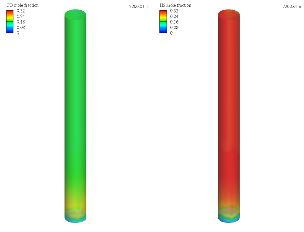
Figure 2: Contours of CO and H2 Mole Fraction in the DRM reactor.
Modeling Instructions
Dry Reforming of Methane (DRM) Reactor Simulation Setup
The user is expected to have gone through basic Barracuda training already Barracuda Virtual Reactor New User Training | CPFD Software (cpfd-software.com).
- Download the support files provided along with this post.
- Unzip the support file and place it in the working directory setup for this DRM project.
- Open a new Barracuda session.
- From the File menu, choose Open Project. Navigate to the working directory and select DRM.prj.
The project file has already been setup with the appropriate
- Grid.
- Base Materials.
- Particles.
- Initial Conditions
- Fluid ICs.
- Particle Species.
- Boundary Conditions
- Pressure BCs.
- Flow BCs.
The chemistry setup for this project, which is already setup, is described in detail below.
Chemistry
Rate and Thermodynamic Coefficients
The reaction kinetics described above need to be converted into a format that is acceptable for inputting into Barracuda.
- Under Chemistry select Rate Coefficients. Click Add to bring up the Chemistry Coefficient Editor (Figure 3). Volume-Average, which is the default reaction type, is used for kinetic constants k1,to k5; and other thermodynamic constants KCH4, KH2O, KCO2, KCO, KH2, KP1, KP2, KP3, KP4 and KP5.
- Reaction kinetic constant k1 will be first input into Barracuda. The units of k1 are mol/kgcat ·sec these need to be converted to mol/m3 ·sec in the Chemistry Coefficient Editor as shown in the following steps.
- Enter 1.29×10⁶ for CO in the Chemistry Coefficient Editor. Leave Type set to Arrhenius Chem Rate.
- Click on Particle dependence in the Chemistry Coefficient Editor.
- In the Particle dependence window, from the Project Materials List add Ni to the Materials List. For Material coefficient type select mass.
- Click OK to close the Particle dependence window.
- Select Mass unit as kg/m3 in the Chemistry Coefficient Editor.
- Divide k1 by θf. Where θf is the volume of fluid in a given control volume.
- To do this put -1 in for C4 in the Chemistry Coefficient Editor.
- The value in the exponential in k1 is divided by the universal gas constant R = 8.314 KJ/Kmol ·K.
- Enter 12,276.30 for E.
- Optional: Add units mol /m3 ·sec in the comment box.
- Reaction kinetic constant k1 will be first input into Barracuda. The units of k1 are mol/kgcat ·sec these need to be converted to mol/m3 ·sec in the Chemistry Coefficient Editor as shown in the following steps.
- Repeat step 1 and enter all remaining rate constants in the Rate Coefficients editor.
- All the remaining thermodynamics constants are in an acceptable format for inputting into Barracuda and can be entered directly in the Rate Coefficients editor.
- Remember to divide the value in the exponent by the universal gas constant R = 8.314 KJ/Kmol ·K.
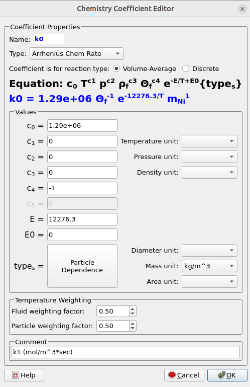
Figure 3: Rate Equations for DRM Reactor Simulation.
Reactions
To finish setting up chemistry portion of this simulation the DRM, RWSG, MD, SG and BR reactions need to be entered into Barracuda.
- Under Chemistry select Reactions. Click Add ⇒ Volume-Average: Stochiometric rate equation to bring up the Chemistry Stochiometric Equation Editor.
- Under Equations Units select mol/m3/sec for Reaction rate units and bar for Fluid species units.
- Enter the Stoichiometric reaction for methane reforming as shown in figure 4.
- Enter the rate equation R1 for the stochiometric reaction as shown in the box R00.
- Click OK to close the Chemistry Stochiometric Equation Editor.
- Repeat steps 1 to 4 and enter the remaining reactions namely RWSG, MD, SG and BR.
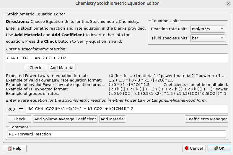
Figure 4: Volume-average Stochiometric Reactions for DRM Reactor Simulation.
Time Controls
- Enter 1e-3 secs for Time Step and 1800 secs for End Time.
- Put 100 secs for Restart Interval.
Visualization Data
- Enter 5 secs for Output file interval.
- Select the Visualization Data for post processing as shown in figure 6.
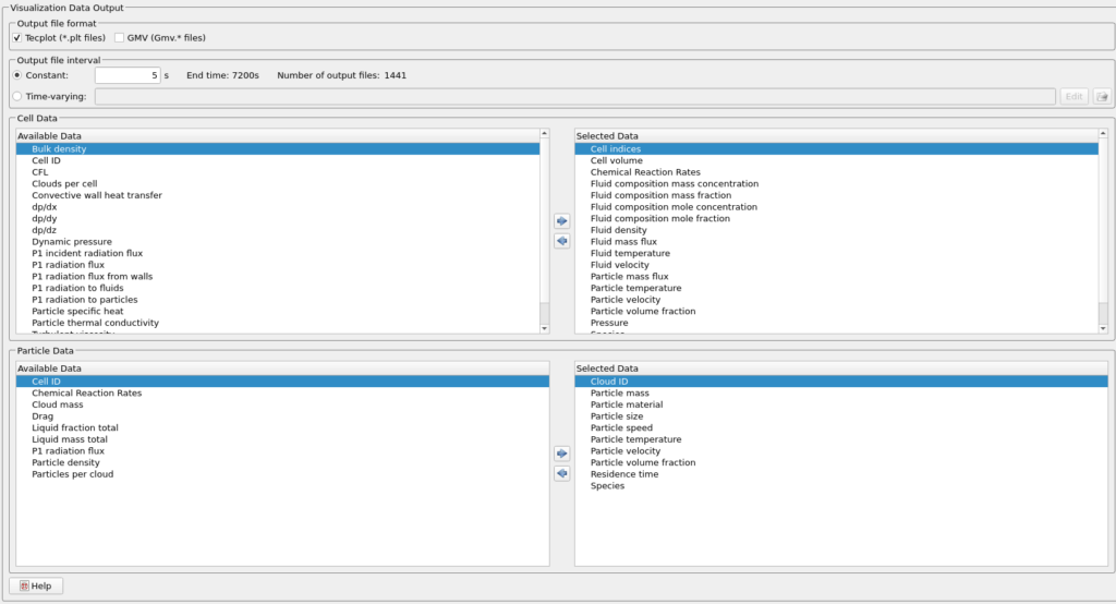
Figure 5: Visualization Data selected for the DRM Reactor Simulation
Run
- Click on Run and then click on Run Solver.
- Select GPU Parallel if you have the required GPU parallel license.
Post Processing DRM Results in Tecplot
The user is assumed to have gone through basic Tecplot training Getting Started With Tecplot For Barracuda® | CPFD Software (cpfd-software.com). So only a few brief steps for post processing the results are explained.
To create the contour plot shown in figure 2 follow the steps shown below.
- In the Barracuda GUI click on Post-Run and then click on View Results.
- Deselect Scatter from the Plot menu.
- Check Contour Box.
- Click on settings beside Contour to open up the Contour & Multi-Coloring Details window.
- From the drop down list select Fluid domain mole fraction CO(G).
- From the drop down list under Color map options select Modified Rainbow – Less Green.
- Click on Set Levels and set the Minimum level to 0, Maximum level to 0.32 and Number of levels to 5.
- Under Color map distribution method change the method to Continuous.
- For contour values at end points enter 0 for Min and 0.32 for Max.
- Click on Close button to close the Contour & Multi-Coloring Details window.
- Click on settings beside Contour to open up the Contour & Multi-Coloring Details window.
- Tecplot frames are used to plot the result for Fluid domain mole fraction H2(G) . The user is expected to have already gone through the training material in “Tecplot for Barracuda – Using frames” (Tecplot for Barracuda – Using Frames | CPFD Software (cpfd-software.com)).
- Click on the outer edge of the current frame and copy it using Ctr + C
- Do a Ctr + V to paste the copied frame
- Select Tile frames from Frame and tile the frames vertically.
- Select Frame ⇒ Frame Linking and then check the boxes for Solution Time, 3D plot view.
- Check the Contour Box.
- Click on settings beside Contour to open up the Contour & Multi-Coloring Details window.
- From the drop down list select Fluid domain mole fraction H2(G).
- From the drop down list under Color map options select Modified Rainbow – Less Green.
- Click on Set Levels and set the Minimum level to 0, Maximum level to 0.32 and Number of levels to 5.
- Under Color map distribution method change the method to Continuous.
- For contour values at end points enter 0 for Min and 0.32 for Max.
- Click on Close button to close the Contour & Multi-Coloring Details window.
- Click on settings beside Contour to open up the Contour & Multi-Coloring Details window.
This concludes the description of the simulation setup process for Application Model: Dry Methane Reforming (DRM) in a Fluidized Bed Reactor in Barracuda Virtual Reactor.
References
Ugarte, P., Durán, P., Lasobras, J., Soler, J., Menéndez, M., & Herguido, J. (2017). Dry reforming of biogas in fluidized bed: Process intensification. International journal of hydrogen energy, 42(19), 13589-13597.
Benguerba, Y., Dehimi, L., Virginie, M., Dumas, C., & Ernst, B. (2015). Modelling of methane dry reforming over Ni/Al2O3 catalyst in a fixed-bed catalytic reactor. Reaction Kinetics, Mechanisms and Catalysis, 114(1), 109-119.
Benguerba, Y., Virginie, M., Dumas, C., & Ernst, B. (2017). Computational fluid dynamics study of the dry reforming of methane over Ni/Al 2 O 3 catalyst in a membrane reactor. Coke deposition. Kinetics and Catalysis, 58, 328-338.