Introduction
Decarbonization of the global energy industry has become a central focus of both academic research and global economic strategy, as the sector strives to meet rapidly increasing demand and environmental protection standards. The expansion of electricity-intensive technologies, such as generative AI data centers, has already exceeded prior energy-consumption projections, spurring the need for reliable, efficient low-carbon power sources. Advances in nuclear technology, particularly the high-temperature gas-cooled reactor (HTGR), are emerging as leading candidates to meet these high demands, with companies like X-energy raising upwards of 700 million dollars in 2025 [6] for their reactor development, and Kairos Power [5] signing a commercial contract with Google to supply their data centers with 500 MW of power by 2035. Integral to the operation of HTGR’s are unique nuclear fuel kernels known as TRi-structural ISOtropic (TRISO) fuel kernels. TRISO particles are a self-contained kernel of UO2 encapsulated by multiple protective layers of carbon and silicon carbide. The multi-layer structure around each fuel particle forms a containment system capable of retaining fission products under extreme operating conditions, thereby providing an inherently safer fuel source. Additionally, if external systems fail in the energy production process, the fission products remain trapped within the particles, limiting the potentially catastrophic consequences of exposure. TRISO particles can be used at significantly higher temperatures (1600-1800 °C) than traditional nuclear fuels, which risk melting at 1200 °C. The increased temperature threshold of TRISO particles enables higher operating temperatures, leading to higher thermal conversion and efficiency and reducing the risk of fuel meltdowns in emergencies. The high operating temperature capacity of TRISO particles can also be leveraged elsewhere, with the carbon emission free process heat eventually used for hydrogen production, chemical synthesis, industrial heating, and petrochemical processing. These qualities all make TRISO particles a key fuel for the future, with decarbonization and distributed energy systems in mind.
To make a TRISO particle, carbon (C) and silicon carbide (SiC) are deposited in layers on the surface of the fuel kernel over four separate stages. In each stage, inert carrier gas and hydrocarbons/methyl trichlorosilane are fed into a spouted-bed reactor, and the reacting gas is pyrolyzed, forming solid carbon/SiC fines that deposit on the surface of the UO2 fuel kernels. The particles in the reactor mix over time as the inlet gas entrains them, eventually forming a “fountain” structure and spouting above the bed. By changing the gas flow rate, reactor temperature, and feed composition, the deposition reaction can be controlled to meet a desired particle growth rate. The design of the TRISO reactor directly impacts the quality of the particles, which must meet rigorous specifications in terms of size, density, layer thickness, and composition. The characteristics of the produced particles are governed by complex multiphase hydrodynamic phenomena occurring during the fabrication process, and experimental investigations of these systems are often limited in resolution, as a deep understanding of heat transfer and reaction kinetics may not be readily captured. Additionally, experimentation is prohibitively expensive to carry out, particularly at high temperatures that match those of operation. Computational fluid dynamics provides a uniquely powerful tool to analyze TRISO systems in a time-efficient and cost-effective manner, and Barracuda Virtual Reactor provides a solution that accurately models and optimizes the hydrodynamics, heat transfer, species transport, and reactions occurring in TRISO reactors from lab to production scale while maintaining full physics fidelity.
In this application model, Barracuda is used to model the production of TRISO particles in a spouted bed reactor, with discussions regarding the model definition, included reactions, key results, and model inputs to come below.
Model Definition
The modeled domain and all of its boundary conditions are shown in Figure 1 below. The simulated reactor is a 3D spouted bed, with an inlet diameter of 8 mm, a bottom diameter of 20 mm, a top diameter of 100 mm, a total height of 250 mm, and a cone angle of 60°. The reactor geometry (based on the work of Liu 2024 [2]) is captured in a grid of 74,000 cells. The model exemplifies the use of a compressible domain, with a mixture of argon and acetylene gases introduced through the inlet flow BC. The gas mixture is fed at 300 K and a velocity of 26 m/s and is quickly heated by convection with the thermal walls, which are set to 1273 K. Initialized above the gas inlet is 0.35 kg of UO2 particles with a uniform diameter of 1.5 mm and a total particle inventory of 18,500. The particles have a very high density (10800 kg/m3) and are assumed to be perfectly spherical. As gas is fed into the system, a high-pressure zone forms in the inlet tube below the bed of particles, eventually building up enough pressure to drive gas through the bed. The high-velocity gas entrains UO2 particles, causing the bed to spout, and drag forces imparted on the particles are calculated using the Beetstra drag model. The gas exits the system from the outlet pressure BC at the top, which is set to atmospheric pressure and 1273 K. To more accurately model dense particle flows in this simulation, the Elastic Collision model was selected. This model provides a more complete calculation of particle stress by accounting for viscous/shear stress, using the full stress tensor. In the Elastic Collision model, shear stress is directly scaled by a tunable parameter known as the angle of internal friction, with a value of 0 chosen for this simulation. The angle of internal friction controls how much shear stress a group of particles can sustain, with high values associated with a more friction-dominated regime and low values associated with more fluid-like behavior. As gas is fed into the reactor, several discrete and volume-average reactions occur, most notably the pyrolysis of acetylene, and the consequent deposition of carbon (1050 kg/m3) on the surface of the UO2 fuel kernels. Over time, the deposited layer thickness continues to grow as the simulation runs for a total of 60 seconds.
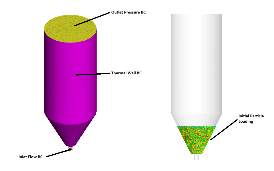
Figure 1: Spouted Bed Reactor Geometry and Boundary Conditions
Reaction Kinetics
The reaction set in this simulation comprises 7 volume-average homogeneous reactions, along with two discrete reactions that account for the direct deposition of carbon as part of the stage one process. The reactions are based on the work of Khan 2008 [3], and the main reaction pathways are shown below.
$$ C_2H_2 + H_2 \rightarrow C_2H_4 \quad \text{(1)} $$
$$ C_2H_4 \rightarrow C_2H_2 + H_2 \quad \text{(2)} $$
$$ C_2H_2 + 3H_2 \rightarrow 2CH_4 \quad \text{(3)} $$
$$ 2CH_4 \rightarrow C_2H_2 + 3H_2 \quad \text{(4)} $$
$$ C_2H_2 \rightarrow 2C(s) + H_2 \quad \text{(5)} $$
$$ C_2H_2 + C_2H_2 \rightarrow C_4H_4 \quad \text{(6)} $$
$$ C_4H_4 \rightarrow C_2H_2 + C_2H_2 \quad \text{(7)} $$
$$ C_4H_4 + C_2H_2 \rightarrow C_6H_6 \quad \text{(8)} $$
$$ C_6H_6 \rightarrow 6C(s) + 3H_2 \quad \text{(9)} $$
The set of reactions above describes a reduced yet physically representative pathway for acetylene pyrolysis, which was specifically chosen to minimize the number of included radical reactions while ensuring that all key products and reaction pathways are represented. The model captures hydrocarbon interconversion and growth via acetylene/ethylene chemistry (Reactions 1–2), methane formation and decomposition (Reactions 3–4), growth of larger hydrocarbons via vinylacetylene and benzene formation (Reactions 6–8), and solid carbon formation (Reactions 5 and 9). The core acetylene pyrolysis step (Reaction 5) produces solid carbon, which, in practice, is responsible for soot formation and subsequent deposition onto fuel kernels, while the methane reactions were included to include hydrogen’s role in suppressing pyrolysis and stabilizing intermediate species in the model. Additionally, acetylene has been shown to polymerize and form larger hydrocarbons (Reactions 6 and 8), which can either decompose back into smaller molecules (Reaction 7) or into solid carbon, providing a second pathway for deposition. Overall, this mechanism captures the competition between gas-phase growth reactions and the key deposition reactions that drive TRISO particle production.
The rate expressions and rate constants for the homogenous gas-phase reactions are shown below. Two discrete reactions are included in this application model and will be discussed in detail in the Modeling Instructions section of this post.
\begin{aligned}
R_1 &= k_1 [C_2H_2] [H_2]^{0.36} \\
k_1 &= 4.4 \times 10^3 \exp\!\left(\frac{-12388.7}{T}\right) \\[6pt]
R_2 &= k_2 [C_2H_4]^{0.5} \\
k_2 &= 3.8 \times 10^7 \exp\!\left(\frac{-24955.8}{T}\right) \\[6pt]
R_3 &= k_3 [C_2H_2]^{0.35} [H_2]^{0.22} \\
k_3 &= 1.4 \times 10^5 \exp\!\left(\frac{-18041.9}{T}\right) \\[6pt]
R_4 &= k_4 [CH_4]^{0.21} \\
k_4 &= 8.6 \times 10^6 \exp\!\left(\frac{-23426.2}{T}\right) \\[6pt]
R_6 &= k_6 [C_2H_2]^{1.6} \\
k_6 &= 1.2 \times 10^5 \exp\!\left(\frac{-14517.7}{T}\right) \\[6pt]
R_7 &= k_7 [C_4H_4]^{0.75} \\
k_7 &= 1.0 \times 10^{15} \exp\!\left(\frac{-40317.5}{T}\right) \\[6pt]
R_8 &= k_8 [C_2H_2]^{1.3} [C_4H_4]^{0.6} \\
k_8 &= 1.8 \times 10^3 \exp\!\left(\frac{-7758}{T}\right) \\[10pt]
\end{aligned}
Results and Discussion
To validate the kinetic model used in this simulation, experimentally determined outlet gas mole fractions [1] and an experimental growth rate [4] were used for comparison. The key time-averaged outlet gas mole fractions are shown below in Figure 2. The Barracuda-predicted outlet mole fraction of C2H2 closely matches the experimental results, differing by only 1%, while predictions of H2 and C6H6 show reasonable agreement. By matching the outlet compositions, the reaction kinetics were considered validated at the reaction temperature (1273K) and specified feed gas composition. The average outlet mole fraction values were recorded after 10 seconds of simulation, at which point the outlet compositions had reached steady state. Matching the outlet mole fractions was a consequence of matching the experimental particle growth rate, and the method used to model particle growth is explained further below in the Chemistry section.
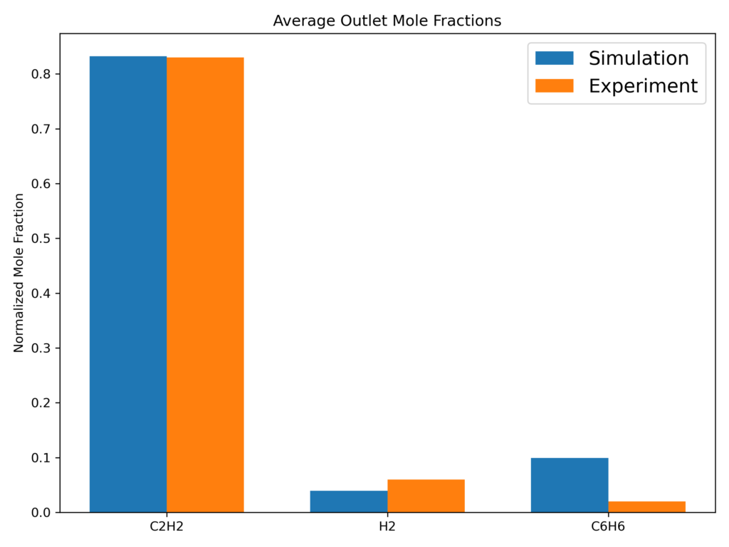
Figure 2: Time Averaged Key Outlet Gas Mole Fractions.
In addition to matching the outlet mole fractions, the referenced experimental growth rate was closely matched in Barracuda (CPFD uses information from the available literature for application model development, but does not independently verify its accuracy). Plots showing layer thickness growth and layer mass growth are shown below (Figures 3 and 4). The two plots present the time evolution of particle growth from two perspectives: geometric-based layer thickness and deposited layer mass. In Figure 3, the y-axis represents the deposited carbon layer thickness (in mm) as a result of the deposition reactions, while Figure 4 represents the deposited mass of carbon (in mg) on the fuel kernel. Both layer thickness and mass deposition vary over time, resulting in two plots that track the growth rate of layer diameter and mass addition over the total length of the simulation. Both the layer thickness and deposited mass were averaged across all particles at each time step over 60 seconds of runtime, yielding a global average growth rate and providing a general idea of how the reactions were progressing. This ensures that the data is representative of a system-wide mean particle instead of an individual particle.
Overlayed on each graph are three reference lines: an orange linear fit line representing the initial particle growth rate in the first second of runtime, a red line representing the steady state stage particle growth rate after 15 seconds of simulation time, and a green line representing the global average growth rate across the entire simulation. The slope of each line is equal to the growth rate (mm/s or mg/s) of TRISO particles for the specific time regime of operation.
Based on observing the orange initial slope reference line, the slope at t<=1 is much higher than at any other point in the simulation. In this initial transience, both thickness and layer mass increase rapidly, which can be explained by the reaction kinetics. This regime is characterized by high reactant availability and low diffusional resistance, allowing the deposition reactions (reactions 5 and 9) to proceed without transport limitations or product inhibition. Initially, the rate of deposition solely depends on the concentration of C2H2 (refer to Figure 12), as little hydrogen has yet been produced in the system. There is an abundance of fresh acetylene, with no side products to inhibit deposition, and diffusional resistance is at its lowest due to low product concentrations. This results in an increased growth rate during the first few seconds resulting in a steep, linear slope observed initially in Figures 3 and 4. While the first few seconds of initial transience may seem irrelevant in the much longer full TRISO deposition stage, it explains the importance of including a full set of kinetics and not simply just the deposition reactions as is commonly done in many simulation studies. By only including the deposition steps, the affects of competing reactions are lost, and deposition will progress unchecked. The resulting growth rate represented in this case by the orange line will be a significant overestimate and an inaccurate representation of physical systems.
As the stage one deposition proceeds, the concentration of produced H2 quickly rises as a pyrolysis product, and several side reactions that inhibit the overall rate of deposition begin to take place. Acetylene, a highly reactive triple-bonded carbon molecule, when fed into the reactor, reacts with hydrogen (Reactions 1 and 3), forming methane and ethylene instead of pyrolyzing. Consequently, the deposition rate decreases and eventually reaches a quasi-steady state rate after about 15 seconds, as indicated by the red reference line on both plots. Many common modeling approaches, such as CFD-DEM, are typically run for only a few seconds of physical simulation time due to high computational overhead, and hence, the system’s transition to a steady-state deposition is overlooked. Because of this, many results reported in academic studies are not truly representative of sustained operation, and a steady state deposition rate is not recorded.
In this application model, using Barracuda, the transition region between initial, chemistry-dominated transience and steady-state operation is captured, with the transition region serving as an indication of how fast the system can reach normal operating conditions. By the time the system is well within steady-state (t>30 s), the layer growth rate stabilizes around 0.1 micron per second, which is of the same order of magnitude as the experimentally determined growth rate. As mentioned previously, the kinetics were primarily tuned to match the experimental deposition rate, and the outlet compositions in Figure 2 consequently matched experimental values.
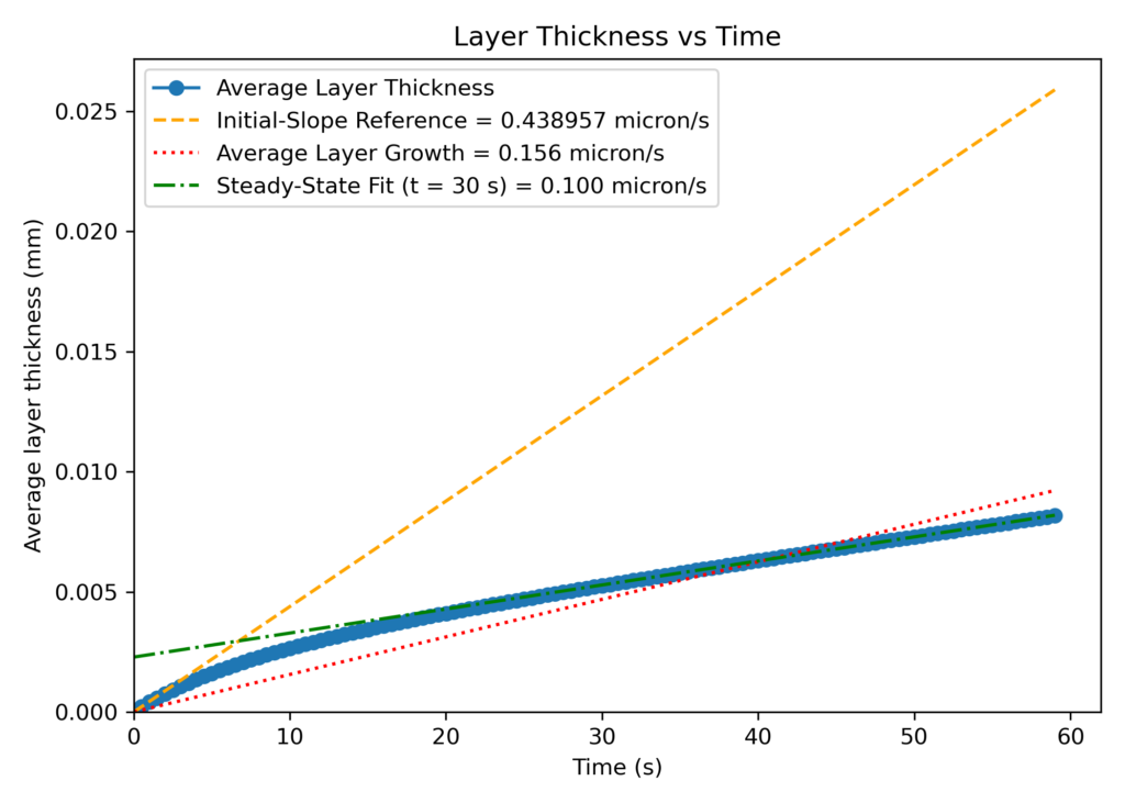
Figure 3: Particle Layer Thickness Over Time.
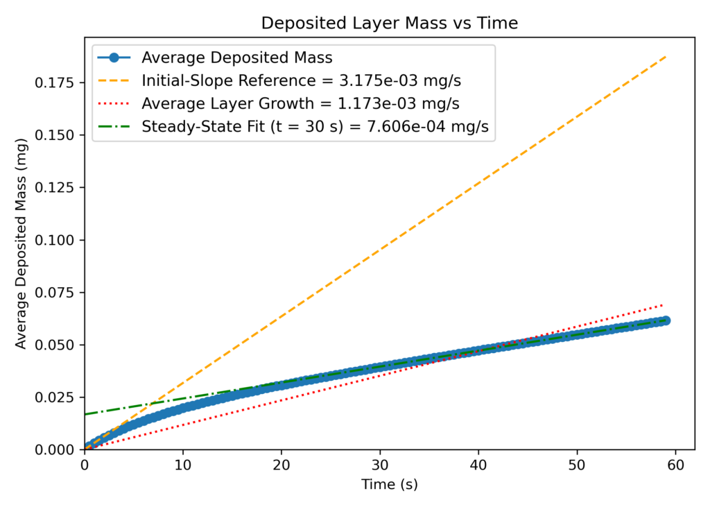
Figure 4: Particle Layer Mass Evolution Over Time.
Figure 5: Particle Size Growth Over Time
The particle size growth animation in Figure 5 above from the Barracuda simulation provides a spatial and time-resolved perspective that directly reinforces the trends observed in the growth plots (Figures 3 and 4). Initially, particles are shown to exhibit faster, uniform growth rates when exposed to high initial concentrations of acetylene, consistent with the steep growth rate observed in the plots. During this time, particles grow more uniformly, and regions of faster growth indicated by lighter colors on the plot are not yet visible. As time progresses in the animation beyond 3 seconds, greater heterogeneity in particle size is observed. Particles near the bottom of the reactor are observed to grow faster because of the abundance of fresh acetylene in this area.
Some particles are shown to grow faster under local flow conditions, mirroring the gradual reduction in the overall growth rate and the curvature of the thickness/mass vs. time plots. This visual evolution aligns most strongly with the intermediate regime in the plots, as the system transitions to steady state. Particles experience varying exposure to fresh reactants, and the coating process becomes increasingly limited by fluid transport and competitive kinetics. By later stages in the animation (t>10 seconds), the growth rate appears more uniform, but not in the absolute layer thickness, reflecting the steady-state deposition regime in the layer growth plots.
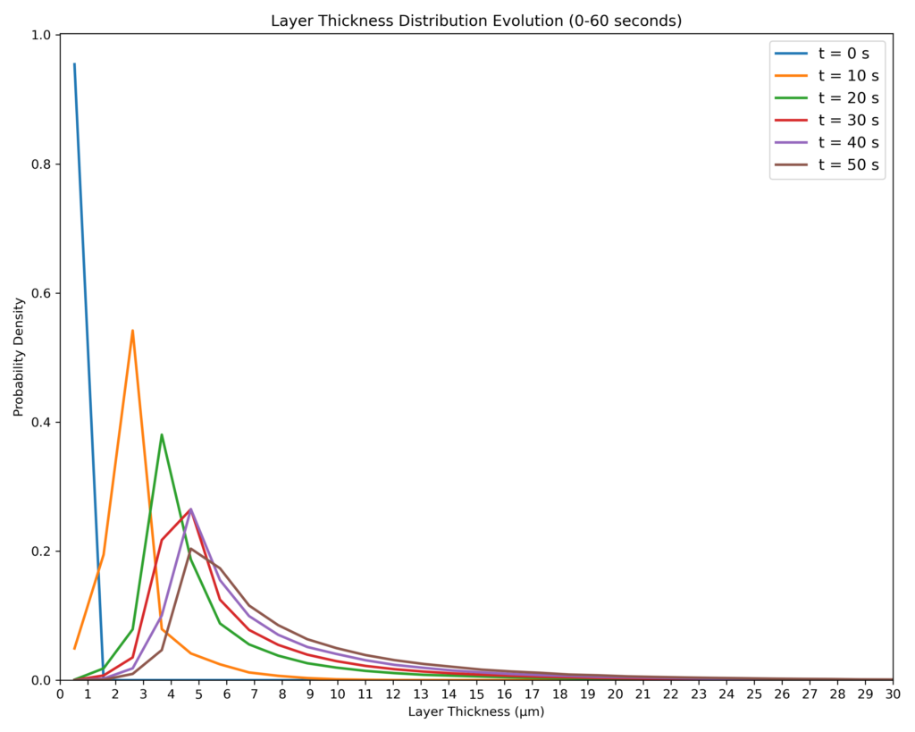
Figure 6: Probability Density Function Across Simulated Stage Time.
Figure 7: Entrainment Difference Between Beginning and End Stage Simulations
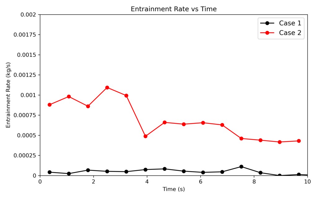
Figure 8: Particle Entrainment Comparison at t=0 and t=18 minutes.
To quantify the rate of entrainment, the mass flow of particles leaving the reactor was recorded, and the rate of particle exit is shown above in Figure 8. The entrainment rates from the reactors were compared over 10 seconds of simulation time, with the red line corresponding to the end stage simulation and the black line corresponding to the beginning stage. The rates of entrainment in the end stage deposition are shown to increase by several orders of magnitude. Further extrapolating to later stages, after additional mass is deposited, and the density continues to decrease, the rates of entrainment will still rise, leading to heavy losses if the reactor’s operating conditions do not account for this. In this context, Barracuda can be used to identify the underlying cause responsible for entrainment, such as local flow conditions and particle size characteristics. Additionally, process operating conditions can be varied in order to confidently understand how changes in reactor operation affect deposition rates and entrainment losses simultaneously.
Modeling Instructions
The user is expected to have already gone through basic Barracuda training: Barracuda Virtual Reactor New User Training | CPFD Software (cpfd-software.com).
- Download the following support files: Beginning Stage TRISO for the beginning stage simulation, and End Stage TRISO for the end stage simulation.
- Unzip the support file and place it in the new folder.
- Open a new Barracuda session.
- From the File menu, choose Open Project. Navigate to the working directory and select the project file.
- Click on Setup Grid -> 3. Generate Grid.
The project file has already been set up with the appropriate:
- Grid
- Base Materials.
- Particles.
- Initial Conditions
- Boundary Conditions
- Heat Transfer
- Chemistry Setup
- Post Processing
The reaction kinetics for this project, which are already set up under the chemistry section in the project file, are described below.
Chemistry
Rate Coefficients
Each reaction of the 9 included homogeneous (1-4, 6-8) and discrete (5,9) has rate constants in the Arrhenius form, requiring a pre-exponential coefficient and an activation energy to be specified. The following set of instructions mirrors how a user would set up rate constant k1 (see Figure 9) in Barracuda’s Chemistry Coefficient Editor.
- Under Chemistry, select Rate Coefficients. Click Add to bring up the Chemistry Coefficient Editor. Volume-Average, which is the default reaction type, is used for this rate constant.
- Ensuring that the Arrhenius Chem Rate is selected, enter the following parameters.
- From (Khan 2008), enter the given pre-exponential factor (4400 s-1) into the c0 variable slot.
- Also from (Khan 2008), multiply the activation energy (103 kJ/mol) by 1000 J/kJ, and divide the resulting value by the universal gas constant (8.314 J/mol*K).
- Input the previous value (12388.7 K) into the E variable slot and finish with Ok.
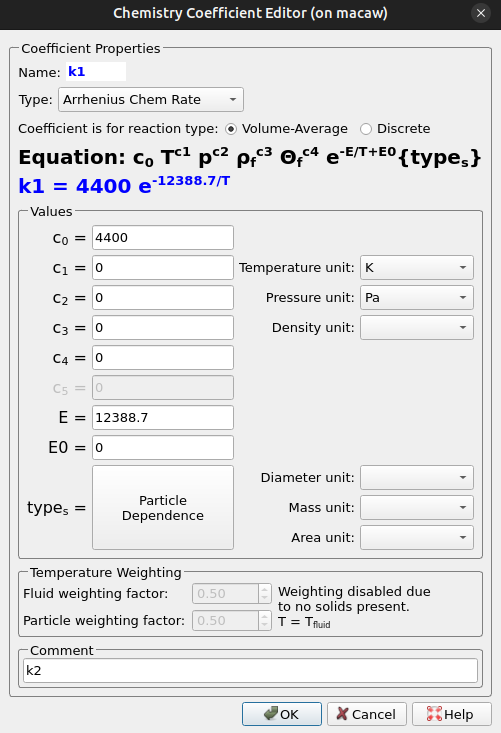
Figure 9: k1 Rate Constant Expression
The remaining volume average reactions are specified following a similar procedure. Reactions 5 and 9 are discrete reactions, and a user-defined constant is needed. The rate constants are both formatted similarly, and the rate constant for reaction 5 (k0) is shown below in Figure 10. For reactions 5 and 9, a tunable parameter, “S,” the scavenging coefficient, directly controls the rate at which solids are deposited on the surface of the TRISO particles and is included in the rate constant expression. With the deposition rate controlled by the scavenging coefficient, the deposition of solids onto the surface of the intialized UO2 fuel kernels, formed from reactions 5 and 9, is handled automatically by the Barracuda solver as part of the calculation. The pre-exponential constant k is derived from the work of (Khan 2008), and formatted in a similar fashion as in k1. The scavenging coefficient, which is multiplied by the pre-exponential term, accounts for the velocity difference between the fluid and particle species, scaling the deposition accordingly. This method simplifies the mechanism by which particles pick up pyrolysis soot in the reactor, thereby controlling the rate of deposition to the specified experimental value.
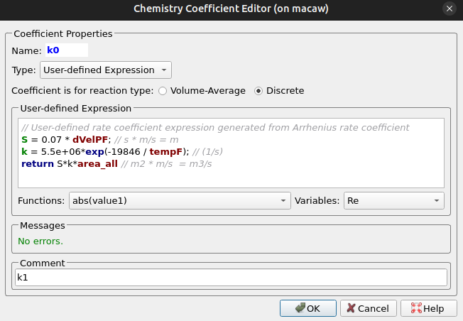
Figure 10: Reaction 5 Rate Expression and Rate Constant (k0).
Reactions
The included reaction set is comprised of 9 reactions, 7 of which are volume-average reactions. The following instructions mirror how a user would set up reaction 1 from (Khan 2008) in Barracuda.
- Navigate to Chemistry, Reactions, and click Add, Volume-Average: Stoichiometric rate-equation to bring up the Chemistry Stoichiometric Equation Editor.
- Under equation units, select mol/m3/s for Reaction rate units and mol/m3 for Fluid species units.
- Enter the stoichiometric equation for reaction 1 as shown in Figure 11.
- In the R00 box, enter the corresponding rate of reaction for reaction 1 as shown in Figure 11.
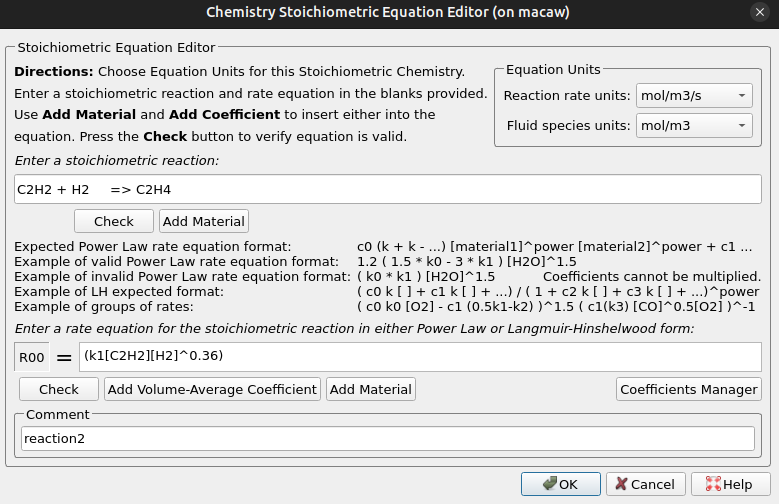
Figure 11: Reaction 1 Stoichiometric Equation Editor
Two of the included reactions are discrete and require special specification in the Chemistry editor. The first discrete reaction is reaction 5, in which acetylene pyrolyzes, producing carbon fines and hydrogen gas. The discrete reaction as entered in Barracuda is shown below in Figure 12. The reaction rate units are chosen as mol/s, and the fluid species units are mol/m3. The rate expression from (Khan 2008) is entered here as k0, which refers to the user-defined rate coefficient in Figure 10. The rates included in the specification indicate that 2 moles of carbon are yielded from one mole of acetylene reacting, and 1 mole of hydrogen is produced for 2 moles of carbon.
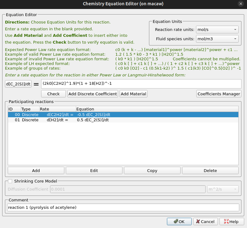
Figure 12: Reaction 5 Discrete Reaction Editor
Time Controls
- Select 1e-04 as the Time Step and 30 seconds as the End Time.
- Select 1s for the Restart Interval.
Visualization Data
The following instantaneous and time-average visualization data are selected for all necessary data post-processing.
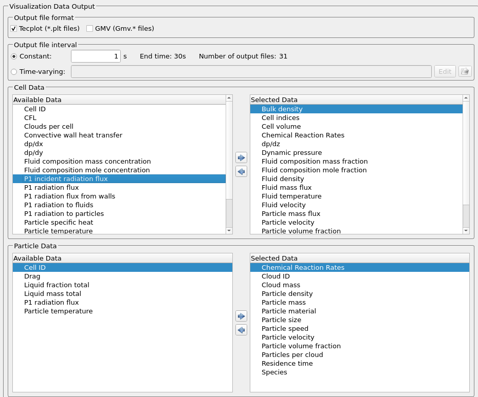
Figure 13: Selected Visualization Data in Barracuda
Run
- Click on Run and select Run Solver.
- Select GPU Parallel if a GPU license is available.
References
- Chen, Meng, Zhao Chen, Yaping Tang, and Malin Liu. CFD-DEM Simulation of Particle Coating Process Coupled with Chemical Reaction Flow Model. International Journal of Chemical Reactor Engineering, 2021.
- Jiang, Lin, Mofan Qiu, Rongzheng Liu, Bing Liu, Youlin Shao, and Malin Liu. CFD-DEM Simulation of High Density Particles Fluidization Behaviors in 3D Conical Spouted Beds. Particuology, vol. 88, 2024, pp. 266–281.
- Khan, Rafi Ullah, Siegfried Bajohr, Frank Graf, and Rainer Reimert. Modeling of Acetylene Pyrolysis under Steel Vacuum Carburizing Conditions in a Tubular Flow Reactor. Molecules, vol. 12, 2007, pp. 290–296.
- Liu, Malin, Meng Chen, Tianjin Li, Yaping Tang, Rongzheng Liu, Youlin Shao, Bing Liu, and Jiaxing Chang. CFD–DEM–CVD Multi-Physical Field Coupling Model for Simulating Particle Coating Process in Spout Bed. Particuology, vol. 42, 2019, pp. 67–78.
- “Google and Kairos Power Team Up for SMR Deployments.” World Nuclear News, 15 Oct. 2024.
- “X-energy Raises $700M in Latest Funding Round.” American Nuclear Society, 25 Nov. 2025.