
Introduction
Hydraulic fracturing creates the flow path between an unconventional reservoir and the wellbore, but that path only stays open as long as the fracture itself stays propped apart. Once pumping stops and fluid pressure bleeds off, the fracture walls close under the confining stress of the surrounding rock, and without something physically holding the crack open, the newly created flow path collapses along with it. Proppant, typically sand or a manufactured ceramic, is carried into the fracture in the fracturing fluid for exactly this reason: it wedges into the open fracture and keeps a permeable channel intact after the treatment ends. Proppant transported into a fracture does not settle evenly along its length. It tends to accumulate more heavily near the injection point, with progressively less reaching the far end of the fracture as pumping continues, a pattern the results below characterize as heel-skewed settling. This uneven distribution directly limits how much of the created fracture area ends up conductive, which in turn limits how much reservoir contact the treatment actually achieves.
Because this settling process happens thousands of feet underground and is effectively impossible to observe directly at full scale, computational fluid dynamics has become one of the primary tools for understanding how proppant moves and settles within a fracture. Several modeling approaches have been applied to the problem. Two-fluid models represent both the fracturing fluid and the proppant as interpenetrating continua with two-way momentum coupling (Zhou et al., 2023), while discrete element methods resolve particle-particle contact directly through soft- or hard-sphere collision models (Zhang et al., 2017; Kou et al., 2018). Each carries a different trade-off between physical fidelity and computational cost, and the choice of method matters for whether a simulation can realistically be run at the scale of an actual fracture treatment.
Barracuda’s multiphase particle-in-cell (MP-PIC) method offers a practical middle ground for this problem. It tracks proppant as discrete Lagrangian parcels, preserving particle size distribution and individual particle trajectories, while representing particle-particle interactions through a continuum stress closure rather than resolving every discrete contact. That combination lets Barracuda capture the settling, bed formation, and bed erosion dynamics that govern proppant placement, without the computational cost of a fully particle-resolved method. Combined with GPU acceleration, this makes it practical to simulate proppant transport at fracture-relevant scales and durations rather than being limited to short, small-domain test cases.
This application model validates Barracuda’s MP-PIC solver against the single-fracture experimental measurements of Zhou et al., 2023, examining proppant settling and bed formation within a single hydraulic fracture, including the use of a non-Newtonian drag correction to account for the shear-thinning behavior of slickwater in the fluid-particle interphase momentum exchange. This validated CFD solution also serves as the training and benchmark data for a Graph Neural Network-based reduced order model (GNN-ROM), a fast surrogate capable of reproducing Barracuda’s predicted proppant distribution at a fraction of the computational cost. Establishing that both the CFD model and its ROM surrogate reproduce this single-fracture benchmark is the necessary first step before extending either to the larger, multi-fracture completions that govern real field-scale proppant placement.
Model Definition
This application model exemplifies the usage of an incompressible flow simulation in Barracuda, validated against the single-fracture experimental measurements of Zhou et al., 2023. The domain represents a single fracture 4000 mm long, 300 mm in height, and 10 mm in width, constructed to mimic the experimental configuration. Flow is injected through three inlets, each 8 mm × 10 mm, on one end of the domain, with three outlets of matching dimensions on the opposite end. Both the continuum fluid and the solid particles are allowed to leave through the outlets. A mesh refinement study was carried out, and the validation case uses a Cartesian-dominant grid with a cell count of 250,000. The model geometry used in Barracuda is shown below (Figure 1).

Figure 1: CFD Domain for single fracture validation case.
Slickwater, with a viscosity of 2.5 mPa·s, is injected into the domain at a velocity of 1.388 m/s, carrying 40/70 mesh proppant at a particle volume fraction of 0.9%, matching the experimental conditions. A full particle size distribution for the 40/70 mesh proppant is defined in the model setup, shown in Figure 2. 40/70 mesh indicates that 90% of sand particles in the mixture fall within a size range of 212 to 425 microns. The fluid-particle interphase momentum exchange uses a custom non-Newtonian drag model, discussed further below, to account for the shear-thinning behavior of slickwater. A subgrid drag correction, based on the analytical wall correction derived by Faxén (1921) and experimentally confirmed by Ambari et al. (1983), is also applied to adjust particle drag as a function of proximity to the fracture wall. A wall friction model is included separately to capture momentum loss from particle sliding and sticking collisions along the fracture walls
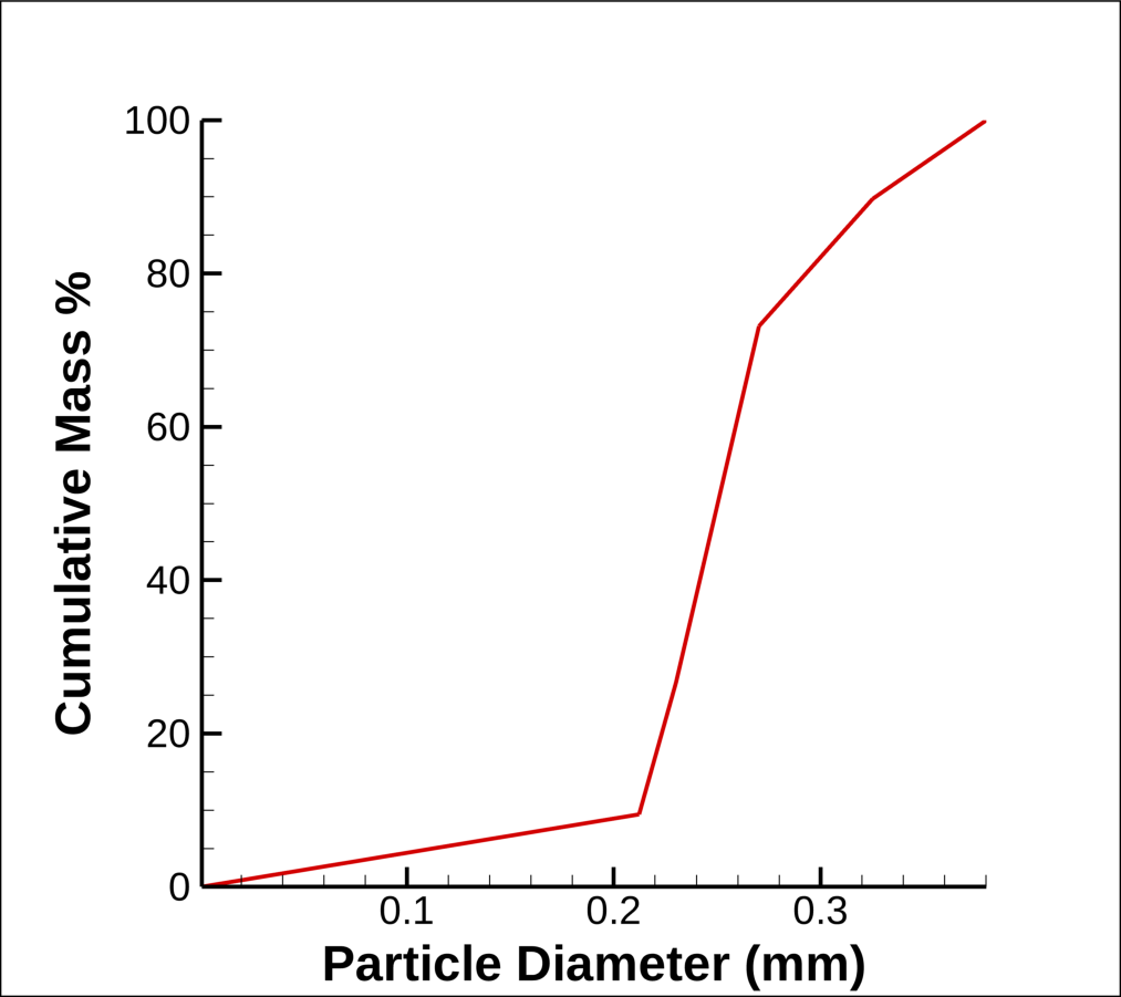
Figure 2: 40/70 Mesh Proppant PSD.
Non-Newtonian Drag Model
In Barracuda, drag models are all defined relative to the Stokes drag law, which describes the drag force acting upon a small spherical particle moving through a viscous fluid at low Reynolds numbers. This case is not universally applicable, and 13 standard drag models are available to choose from in Barracuda. For this simulation, a modified version of the Beetstra drag model, corrected for non-Newtonian fluids following Chhabra (1990), was used to account for the shear-thinning nature of slickwater. The Chhabra-Beetstra drag model was specified using a user-defined drag expression, shown below in Figure 3. To define this drag model for slickwater, several power-law based parameters were adopted.
For a Newtonian fluid, the shear stress experienced is linearly proportional to the rate of shear, where \(\tau\) is the shear stress (in Pa), \(\mu\) is the dynamic viscosity (in Pa\(\cdot\)s), and \(\dot{\gamma}\) is the shear rate (in s\(^{-1}\)).
\begin{equation}
\tau = \mu \, \dot{\gamma}
\end{equation}
For non-Newtonian fluids, however, the relationship between shear stress and shear rate is non-linear, and it becomes beneficial to rewrite the stress relationship in a different manner. Shear rate \(\dot{\gamma}\) is defined as the velocity gradient perpendicular to the direction of flow. For flow in the \(x\)-direction with a velocity field \(u(y)\), the shear rate is given by:
\begin{equation}
\dot{\gamma} = \frac{du}{dy}
\end{equation}
In many non-Newtonian fluids, the shear stress due to viscosity can be modeled more specifically as a power-law model:
\begin{equation}
\tau_{xy} = K \left( \frac{du}{dy} \right)^n
\end{equation}
where \(\tau_{xy}\) is the shear stress, \(K\) is the consistency index (units Pa\(\cdot\)s\(^n\)), \(n\) is the flow behavior index (dimensionless), and \(\frac{du}{dy}\) is the shear rate.
To ensure that the shear stress \(\tau_{xy}\) always has the same sign as \(\frac{du}{dy}\), this expression is often rewritten to preserve sign information explicitly:
\begin{equation}
\tau_{xy} = K \left| \frac{du}{dy} \right|^{n-1} \frac{du}{dy}
\end{equation}
From this, we can define the effective viscosity \(\mu_{\text{eff}}\) as:
\begin{equation}
\mu_{\text{eff}} = K \left| \frac{du}{dy} \right|^{n-1}
\end{equation}
So the shear stress can be written in a Newtonian-like form using the effective viscosity:
\begin{equation}
\tau_{xy} = \mu_{\text{eff}} \, \frac{du}{dy}
\end{equation}
This expression shows that the effective viscosity depends on the shear rate. When \(n = 1\), \(\mu_{\text{eff}} = K\), and the fluid behaves as a Newtonian fluid with constant viscosity.
A characteristic shear rate around a spherical particle can be approximated by:
\begin{equation}
\dot{\gamma} = \frac{|u_f – u_s|}{d_p}
\end{equation}
Substituting this characteristic shear rate into the effective viscosity expression yields:
\begin{equation}
\mu_{\text{eff}} = K\left(\frac{|u_f – u_s|}{d_p}\right)^{n-1}
\end{equation}
The classical particle Reynolds number for a spherical particle in a Newtonian fluid is defined as:
\begin{equation}
Re_p = \frac{\rho_f d_p |u_f – u_s|}{\mu_f}
\end{equation}
Replacing the Newtonian viscosity in the Reynolds number definition with the effective viscosity, we have:
\begin{align}
Re_{ow} &= \frac{\rho_f d_p |u_f – u_s|}{\mu_{\text{eff}}} \\
&= \frac{\rho_f d_p |u_f – u_s|}{K\left(\frac{|u_f – u_s|}{d_p}\right)^{n-1}} \\
&= \frac{\rho_f d_p^n |u_f – u_s|^{2-n}}{K}
\end{align}
Therefore, the modified Reynolds number for a power-law non-Newtonian fluid is:
\begin{equation}
Re_{ow} = \frac{\rho_f d_p^n |u_f – u_s|^{2-n}}{K}
\end{equation}
Additionally, a dimensionless viscosity ratio can compare the non-Newtonian value to that of a reference Newtonian fluid:
\begin{align}
\frac{\mu_{\text{eff}}}{\mu_f} &= \frac{K\left(\frac{|u_f – u_s|}{d_p}\right)^{n-1}}{\mu_f} \\
&= \frac{K|u_f – u_s|^{n-1} d_p^{1-n}}{\mu_f}
\end{align}
This modified particle Reynolds number, \(Re_{ow}\), is the key result from Chhabra (1990): a drag correlation developed for Newtonian fluids, such as the Beetstra model, remains valid for a power-law non-Newtonian fluid provided it is evaluated using \(Re_{ow}\) rather than the ordinary Reynolds number \(Re\). The non-Newtonian drag coefficient is therefore:
\begin{equation}
C_d(Re_{ow}) = \frac{24}{Re_{ow}}F_{ow}(\epsilon, Re_{ow})
\end{equation}
where \(F_{ow}(\epsilon, Re_{ow})\) is the standard Beetstra correction function evaluated at \(Re_{ow}\).
Barracuda, however, builds its internal drag force using the ordinary Newtonian Reynolds number \(Re\) as the basis for its correction function \(F(\epsilon, Re)\), not \(Re_{ow}\). The Chhabra-corrected drag model therefore cannot simply set \(F(\epsilon, Re)\) equal to \(F_{ow}(\epsilon, Re_{ow})\); the two must instead be related so that both formulations predict the same physical drag force. Equating Barracuda’s internal drag expression to the true non-Newtonian drag force and solving for \(F(\epsilon, Re)\) gives:
\begin{equation}
F(\epsilon, Re) = \frac{Re}{Re_{ow}}F_{ow}(\epsilon, Re_{ow})
\end{equation}
This ratio correction is the logic implemented directly in the user-defined drag expression, shown below in Figure 3.
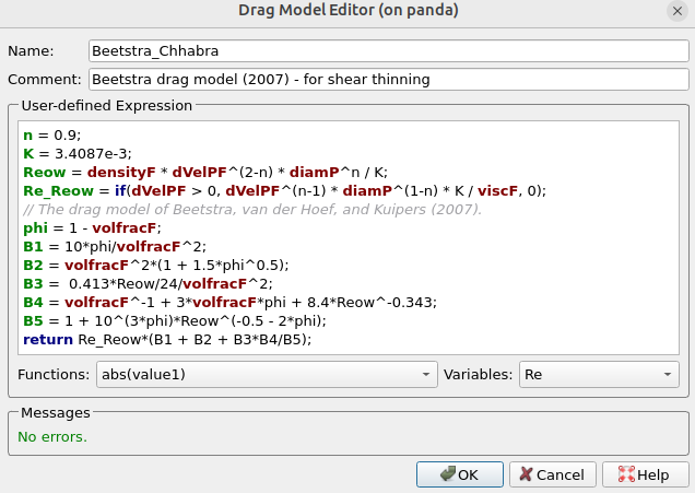
Figure 3: User-defined Non-Newtonian Drag Model
Results and Discussion
Both the CFD model and the GNN-ROM are validated against the single-fracture experimental measurements of Zhou et al., 2023, before either is applied to more complex, field-scale configurations. The GNN-ROM is trained on Eulerian particle volume-fraction fields generated by the validated CFD model at injection velocities of 1.2 and 1.45 m/s. The intermediate case shown here, at 1.388 m/s, is withheld from training entirely and used only for evaluation against the CFD solution and the experimental bed-height measurements, making this a genuine test of the ROM’s ability to generalize rather than an interpolation check on data it has already seen.
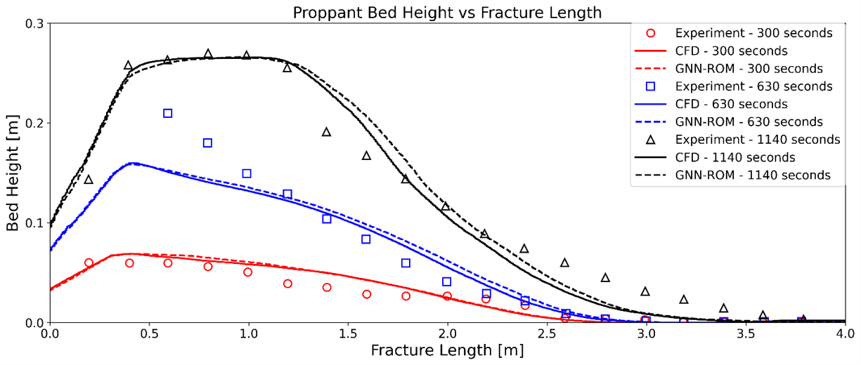
Figure 4: Experimental, CFD, and GNN-ROM proppant-bed-height profiles at 300, 630, and 1140 s. The bed interface was extracted from both CFD and ROM particle-volume-fraction fields using a common threshold of 0.45.
Figure 4 compares the experimental, CFD, and GNN-ROM proppant bed-height profiles at 300, 630, and 1140 seconds for the 1.388 m/s case. These three times capture different stages of bed development. Early on, proppant motion is governed primarily by fluid-particle drag and particle-particle interactions as the bed begins to form. As pumping continues and the fracture fills, frictional contact forces within the already-settled bed become increasingly important in shaping how the bed continues to grow. The CFD solution reproduces the principal evolution seen in the experiment, capturing the transition from a rounded bed profile at 300 seconds to a longer bed with a steeper downstream slope at later times. Some differences in the finer details of the profile curvature remain, due in part to the fact that only a coarse approximation of the experimental particle size distribution was available as an input to the CFD model.

Table 1: Quantitative comparison of single-fracture CFD and GNN-ROM results
The GNN-ROM closely follows the CFD bed-height profiles at all three times shown. As summarized in Table 1, its mean absolute error relative to the experimental measurements stays close to that of the CFD solution itself, and the bed area it predicts differs from the CFD result by only 1.38 to 3.31 percent across the three time steps. Given that this evaluation case was withheld from the GNN-ROM’s training set, this level of agreement indicates the surrogate has learned the underlying transport and settling behavior well enough to generalize to an unseen operating condition, rather than simply reproducing cases it has already been shown. Full details of the GNN-ROM architecture and training methodology are described in Mitra et al. (2026).
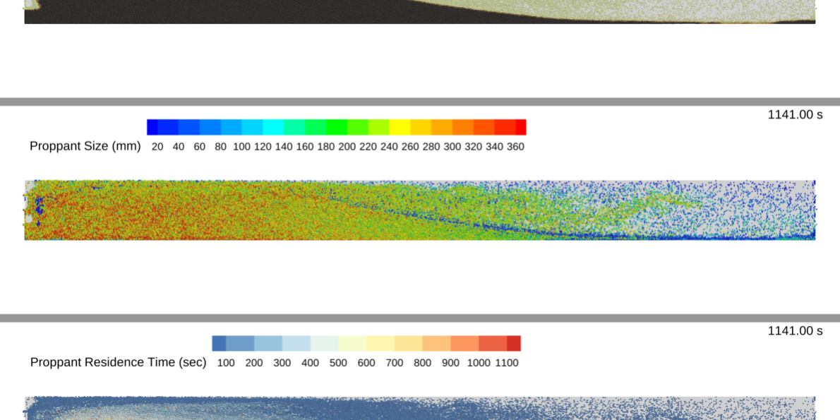
Figure 5 shows an animation of particle volume fraction, particle size, and residence time from t = 0 to 1140 seconds.
Figure 5: Animation of particle volume fraction, particle size, and residence time from t = 0 to 1140 s.
At the start of injection, proppant enters as a dilute, fully mixed suspension that spans the length of the fracture, with particles of all sizes carried together in the fluidized zone near the top of the channel. As pumping continues, particles begin settling out near the inlet, and a packed bed forms and grows steadily along the base of the fracture, developing the characteristic dune shape with a steep face near the inlet and a long, shallow tail extending downstream. The particle size field shows this process is accompanied by size segregation: coarser particles preferentially settle and accumulate in the thick, near-inlet portion of the bed, while finer particles are carried further downstream before settling into the thinning tail. The residence time field shows the bed building from the bottom up, with the oldest particles buried in a continuous layer along the base near the inlet and progressively younger particles settling on top and further downstream as injection continues, consistent with a heel-skewed bed that grows primarily by accretion rather than by redistributing material already at rest.
Modeling Instructions
The user is expected to have already gone through basic Barracuda training, Barracuda Virtual Reactor New User Training | CPFD Software (cpfd-software.com).
- Download the support files provided along with this post.
- Unzip the support file and place it in the working directory set up for this Sand Screen Filtration Performance project.
- Open a new Barracuda session.
- From the File menu, choose Open Project. Navigate to the working directory and select single_fracture_proppant_transport.prj.
The project file has already been set up with the appropriate
- Grid.
- Baffle Definition and passing probability
- Base Materials.
- Initial Conditions
- Fluid ICs.
- Particle Species.
- Boundary Conditions
- Pressure BCs.
- Flow BCs.
Time Controls
- Enter 0.005 secs for Time Step and 1141 secs for End Time.
- Enter 100 secs for the Restart Interval.
Visualization Data
- Enter 2 secs for the Output file interval.
- Select the Visualization Data for post-processing as shown in Figure 6.
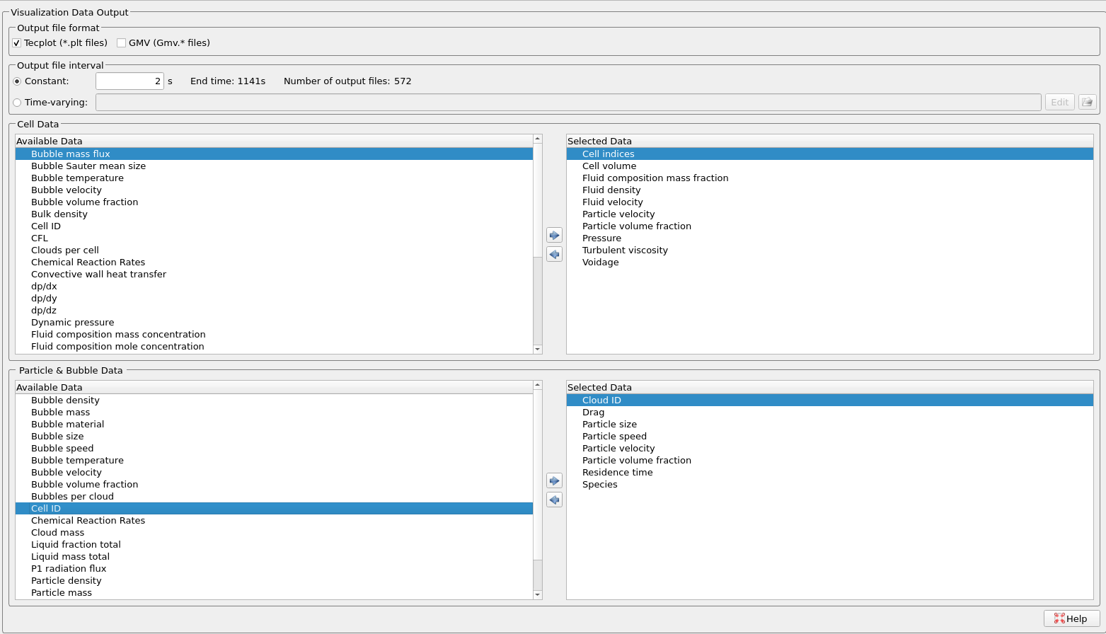
Figure 6: Visualization data selected for post-processing.
Run
- Click on Run and then click on Run Solver.
- Select GPU Parallel if you have the required GPU parallel license.
Post-Processing in Tecplot
The user is assumed to have gone through basic Tecplot training, Getting Started With Tecplot For Barracuda® | CPFD Software (cpfd-software.com). Only a few brief steps for post-processing the results are explained.
To reproduce the animation shown in Figure 5, use the layout file fig5.lay provided in the zipped support file. To load the layout file into Tecplot from the Barracuda GUI:
- Navigate down to Post-Run in the project tree and select either View Results or Launch Tecplot tab.
- In the newly opened Tecplot window, select File –> Load Barracuda Data –> Load Layout, navigate to the directory where the support file was unzipped and saved, and select fig5.lay and click Open. This should then reproduce the view shown in the figure for top and bottom panel animations.
This concludes the description of the Application Model: Proppant Transport in a Single Hydraulic Fracture Using MP-PIC CFD and a Graph Neural Network Reduced-Order Model (GNN-ROM)
References
Zhou, H., Guo, J., Zhang, T., Li, M., Tang, T., & Gou, H. (2023). Eulerian multifluid simulations of proppant transport with different sizes. Physics of Fluids, 35(4).
Zhang, G., Li, M., & Gutierrez, M. (2017). Numerical simulation of proppant distribution in hydraulic fractures in horizontal wells. Journal of Natural Gas Science and Engineering, 48, 157–168.
Kou, R., Moridis, G. J., & Blasingame, T. A. (2018, January). Analysis and modeling of proppant transport in inclined hydraulic fractures. In SPE Hydraulic Fracturing Technology Conference and Exhibition (p. D011S002R001). SPE.
Faxén, H. (1921). Einwirkung der Gefässwände auf den Widerstand gegen die Bewegung einer kleinen Kugel in einer zähen Flüssigkeit. Förf.
Ambari, A., Gauthier Manuel, B., & Guyon, E. (1983). Effect of a plane wall on a sphere moving parallel to it. Journal de Physique Lettres, 44(4), 143–146.
Chhabra, R. P. (1990). Motion of spheres in power law (viscoinelastic) fluids at intermediate Reynolds numbers: A unified approach. Chemical Engineering and Processing: Process Intensification, 28(2), 89–94.
Mitra, S., Karra, S. K., Ramchandran, K., & Parker, J. (2026). Graph neural network reduced-order models for multiphase CFD: Fluidized bed and hydraulic fracturing applications. Proceedings of the ASME Fluids Engineering Division Summer Meeting, FEDSM2026-182699.