
Introduction
While fostering the development of clean energy technologies is a global focus in the scientific community, a large portion of the world still relies on the same resource used in the Industrial Revolution: coal. According to the IEA, 60% of the world’s electricity comes from fossil fuels, with 35% coming from coal combustion [3]. Countries like India and China get the majority of their energy from coal (74.5% and 54%), and several innovative technologies have been employed to deliver the masses with the energy they need. The two most common processes for coal-fired power generation are pulverized coal combustion (PC) and circulating fluidized bed (CFB) combustion. The more common of the two is PC combustion, in which coal is crushed to a fine powder and burned with air over a flame at temperatures around 1300 °C. This process is used in the great majority of coal-fired energy production, but produces many unwanted emissions due to the high temperatures and requires significant downstream gas scrubbing. CFB combustors provide a more robust, flexible, and environmentally friendly energy production process. See Figure 1 for the CFB combustor geometry modeled in this post. In an operating CFB, ash and limestone circulate through the system, fluidized by primary air fed at the furnace floor. Solid fuel is then fed into a dense zone at the bottom of the riser and fluidized. The fuel and ash circulate through the system at varying rates, becoming entrained in the high gas velocities and passing through cyclones at the top of the riser, where they are returned to the bottom. Fuel will combust slowly as it passes through the system several times before achieving complete combustion. The system’s high residence times provide excellent gas-solid mixing and enable efficient burnout of low-reactivity fuels. The fraction of the bed occupied by fuel is very low, with over 95% of the circulating solids being limestone and ash. The relatively uniform composition of the bed results in uniform temperature throughout the furnace and highly efficient heat transfer. The type of fuels used in CFB combustors also provides an advantage to PC combustors. PC combustors require a narrow range of coal fuel, as variations may lead to ignition issues, slagging (molten coal that sticks to the walls), and fouling. CFB combustors can handle a broad range of fuels, such as low-grade and high-ash coals, waste-derived fuels, petcoke, and biomass. This provides an operational advantage, as fuels can be selected based on market conditions without requiring significant changes to the process. Operating temperatures in CFB combustors range from 800 to 900 °C, much lower than in PC combustion, resulting in significant reductions in emissions. Low-temperature combustion and locally reducing reactions in the CFB reduce thermal NOx formation, unlike in PC combustion, where a catalytic selective reduction system is needed to reduce NOx emissions. Additionally, adsorbing agents, such as limestone, are included in the circulating solids to reduce SOx emissions from the system. The limestone is calcined to calcium oxide, which then reacts with SOx, reducing overall emissions. Historically, the major advantage of PC combustion systems has been higher combustion efficiency, but by leveraging economies of scale and recent improvements in CFB design, newer processes can operate in the 450-600 MW range, comparable to PC combustion plants. This application model post will cover the model setup of an industrial-scale CFB combustor simulated in Barracuda and will also discuss the relevant operating conditions, the included reaction set, and the CFB combustor’s key results.
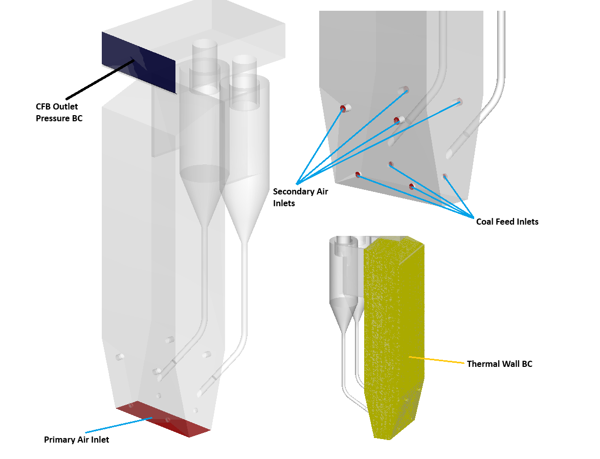
Figure 2: Gas Velocity Streamtraces (m/s)
Model Definition
This application model exemplifies the usage of a compressible domain with volumetric reaction chemistry in Barracuda. The modeled geometry (Figure 1) is derived from a physical 110 MW CFB described by Yang et al. (2023) [9]. The modeled domain is shown in Figure 2, fitted with 4 coal inlets, 4 secondary air inlets, and two cyclones, complete with return diplegs. A bottom-up description of the CFB will follow. The primary air inlet is modeled as the floor of the CFB, with dimensions of 2.4 x 8.70 meters. The riser width then increases to 5.4 meters, remaining at this width for the rest of the riser, another 20 meters, reaching a total riser height of 28 meters. A total of 4 coal inlets are placed at an elevation of 1 meter, all with 0.4 meter I.D.’s. Directly above the coal inlets, a set of 4 secondary air inlets with 0.475-meter I.D.s are placed at 4 meters in elevation. At the top of the riser, two 4-meter I.D. cyclones are fitted, returning solids via two diplegs that exit at an elevation of 2.5 meters. Gas exits the top of the cyclones and flows out of the system at the CFB outlet. In total, 11 boundary conditions are specified throughout the system. Figure 2 also highlights and labels each. A total of 9 flow BCs are specified, one for each coal inlet, one for each secondary air inlet, and a single BC for the primary air inlet. A single pressure BC is defined at the CFB outlet, and a thermal wall BC is applied around the riser to simulate heat loss through the walls of the furnace. Primary air is fed at 11.91 kg/s, with 5.96 kg/s of secondary air supplied through 4 inlets. Air is also supplied to each coal inlet to promote fluidization, with a total flow rate of 0.96 kg/s. The airflow rates were determined based on an excess air ratio of 1.2 and superficial gas velocity from Wu et al (2017) [6]. The coal feed rate, also based on Wu et al. (2017), was calculated to be 2.254 kg/s, with 60,000 kg of ash initially loaded and circulated through the system prior to coal injection. The system is reactive and thermal, with heat capacities varying with temperature. A thermal resistance value is applied for the riser walls to account for heat losses in the system. Ash particles are initialized at an equilibrium temperature of 1123 kelvin, with coal particles being fed at 298 kelvin. Many reactions in the CFB are endothermic, and the heat from circulating ash particles provides the energy needed for them to occur. Secondary air is also fed at 298 kelvin to limit the formation of harmful side products. The particle species modeled in this simulation are bituminous coal feed (containing volatiles) and ash, modeled as devolatilized coal. The composition of coal particles is determined from the proximate and ultimate analysis of the coal type provided in Wu et al’ 2017. The enthalpy of devolatilization is obtained from the heating value provided in Wu 2017. The coal feed is assumed to be perfectly spherical with a uniform diameter of 350 microns. Ash is given a wide particle size distribution from 0-3000 microns, and a Sauter mean diameter of 350 microns to account for larger bed ash and fly ash that is more easily circulated through the system. The Radl-Sundaresan drag model is used to capture the fluid-solid drag interaction for both particle species. A pressure drop of 50 Pa is specified at the outlet, and the inlets are all assumed to operate at atmospheric pressure.
Reaction Kinetics
The kinetic model for the CFB combustion process was derived from several sources, with reactions 1-4, 6-7, 9-12, 14, 16, and 18-19 from Krusch 2018 [1]. Additionally, reactions 5 and 15 are from Wu, 2017; reactions 13, 24, and 25 are from Xie, 2017 [8]; reaction 17 and the discrete reaction for CaO absorption of SO2 are from Xie, 2014[7]. A complete list of sources is provided further below, and a full reaction set is provided in the downloadable support file attached to this post. The reaction set consists of fluid-phase volumetric reactions and discrete reactions that release several volatile species. Two reactions are user-defined and are specified later in this application model post. The full reaction set is shown below, with more details on the different reaction classes to be discussed further in this section.
$$ CO + H_2O \rightarrow CO_2 + H_2 \quad \text{(1)} $$
$$ CO_2 + H_2 \rightarrow CO + H_2O \quad \text{(2)} $$
$$ CH_4 + 1.5O_2 \rightarrow CO_2 + 2H_2O \quad \text{(3)} $$
$$ 2H_2 + O_2 \rightarrow H_2O \quad \text{(4)} $$
$$ CO + 0.5O_2 \rightarrow CO_2 \quad \text{(5)} $$
$$ C(s) + H_2O(v) \rightarrow CO + H_2 \quad \text{(6)} $$
$$ C(s) + CO_2 \rightarrow 2CO \quad \text{(7)} $$
$$ Soot + O_2 \rightarrow CO_2 \quad \text{(8)} $$
$$ HCN + 1.25O_2 \rightarrow NO + CO + 0.5H_2O(v) \quad \text{(9)} $$
$$ HCN + NO + 0.75O_2 \rightarrow N_2O + CO + 0.5H_2O(v) \quad \text{(10)} $$
$$ NH_3 + NO + 0.25O_2 \rightarrow N_2 + 1.5H_2O(v) \quad \text{(11)} $$
$$ NO + CO \rightarrow 0.5N_2 + CO_2 \quad \text{(12)} $$
$$ NO + C(s) \rightarrow 0.5N_2 + CO \quad \text{(13)} $$
$$ NH_3 + 1.25O_2 \rightarrow NO + 1.5H_2O(v) \quad \text{(14)} $$
$$ N_2O + C(s) \rightarrow N_2 + CO \quad \text{(15)} $$
$$ NH_3 + 0.75O_2 \rightarrow 0.5N_2 + 1.5H_2O(v) \quad \text{(16)} $$
$$ H_2S + 1.5O_2 \rightarrow SO_2 + H_2O(v) \quad \text{(17)} $$
$$ C(s) + 0.5O_2 \rightarrow CO \quad \text{(18)} $$
$$ C(s) + O_2 \rightarrow CO_2 \quad \text{(19)} $$
$$ S(s) + O_2 \rightarrow SO_2 \quad \text{(20)} $$
$$ N(s) + 0.5O_2 \rightarrow NO_2 \quad \text{(21)} $$
$$ H(s) + 0.25O_2 \rightarrow 0.5H_2O(v) \quad \text{(22)} $$
$$ O(s) \rightarrow 0.5O_2 \quad \text{(23)} $$
$$ N_2O + CO \rightarrow N_2 + CO_2 \quad \text{(24)} $$
$$ N_2O \rightarrow N_2 + 0.5O_2 \quad \text{(25)} $$
$$ NO + 0.5C(s) \rightarrow 0.5N_2 + 0.5CO_2 \quad \text{(26)} $$
$$ N_2 + O_2 \rightarrow 2NO \quad \text{(27)} $$
A major source of reactants in the CFB combustor comes from the release of volatiles (CO, CO2, CH4, H2, H2S, HCN, and NH3) held within the coal particles. Chronologically speaking, the release of volatiles, modeled as a discrete reaction, marks the beginning of overall reactions in a CFB. The discrete reactions are listed below, and their implementation in Barracuda is shown in Figure 13 of this post. Many reactions occur concurrently in a CFB combustor, but volatile release is by far the fastest, and released volatile species are qucikly oxidized in a number of following reactions.
\begin{gathered}
\frac{d}{dt}[CH_4] = -0.55165\frac{d}{dt}[Volatiles] \\
\frac{d}{dt}[CO] = -0.00028\frac{d}{dt}[Volatiles] \\
\frac{d}{dt}[NH_3] = -0.00337\frac{d}{dt}[Volatiles] \\
\frac{d}{dt}[HCN] = -0.0125\frac{d}{dt}[Volatiles] \\
\frac{d}{dt}[H_2] = -0.00539\frac{d}{dt}[Volatiles] \\
\frac{d}{dt}[H_2S] = -0.02585\frac{d}{dt}[Volatiles] \\
\frac{d}{dt}[CO_2] = -0.40096\frac{d}{dt}[Volatiles] \\
\end{gathered}
Oxygen introduced through primary air oxidizes the released volatiles in reactions 3-5 seen below and in the complete list of reactions further above. The main hydrocarbon (methane), as well as hydrogen and carbon monoxide, are combusted quickly, and a water gas shift reaction also occurs in the system.
$$ CH_4 + 1.5O_2 \rightarrow CO_2 + 2H_2O $$
$$ 2H_2 + O_2 \rightarrow H_2O $$
$$ CO + 0.5O_2 \rightarrow CO_2 $$
$$ CO + H_2O \rightarrow CO_2 + H_2 $$
At the same time, nitrogen-containing volatiles undergo distinct oxidation and reaction pathways (9-12, 14, 16, 24-25, 27), ultimately producing the key pollutants that exit the system. HCN, N2, and NH3 are directly oxidized, as well as reduced with NO or CO in the presence of oxygen. It is important to understand these reactions in order to mitigate NOx formation, which is primarily controlled by staging the oxygen feed between the primary and secondary air inlets. Balancing the primary-to-secondary air ratio can help control the oxygen concentration in the dense bed. Minimizing the amount of oxygen able to oxidize the nitrogenous volatiles in the dense bed can promote a nitrogen reduction pathway instead of the formation of NOx.
\[
\begin{gathered}
HCN + 1.25O_2 \rightarrow NO + CO + 0.5H_2O(v) \\
NH_3 + 1.25O_2 \rightarrow NO + 1.5H_2O(v) \\
NH_3 + 0.75O_2 \rightarrow 0.5N_2 + 1.5H_2O(v) \\[16pt]
HCN + NO + 0.75O_2 \rightarrow N_2O + CO + 0.5H_2O(v) \\
NH_3 + NO + 0.25O_2 \rightarrow N_2 + 1.5H_2O(v) \\[16pt]
N_2 + O_2 \rightarrow 2NO \quad (Thermal \quad NO_x) \\[16pt]
NO + CO \rightarrow 0.5N_2 + CO_2 \\
N_2O + CO \rightarrow N_2 + CO_2 \\
N_2O \rightarrow N_2 + 0.5O_2
\end{gathered}
\]
After the volatiles have left the coal particles, the main component remaining to react is carbon. Char reactions (6-7, 13, 15, 18-19, 26) occur on the surface of coal particles and involve reactions of surface carbon with oxygen, volatiles, pollutants, and intermediate species. These reactions progress over time, and the high residence time of coal in the system per pass allows for adequate gas-solid contacting and eventually, the carbon is completely consumed. Surface carbon is oxidized to form more CO and CO2, but can also react with nitrogen species, further reducing them and decreasing pollutant concentrations. The reactions are shown below.
\[
\begin{gathered}
C(s) + 0.5O_2 \rightarrow CO \\
C(s) + O_2 \rightarrow CO_2 \\
C(s) + H_2O(v) \rightarrow CO + H_2 \\
C(s) + CO_2 \rightarrow 2CO \\[16pt]
NO + C(s) \rightarrow 0.5N_2 + CO \\
N_2O + C(s) \rightarrow N_2 + CO \\
NO + 0.5C(s) \rightarrow 0.5N_2 + 0.5CO_2
\end{gathered}
\]
Additionally, as with surface carbon, other surface species, such as nitrogen and hydrogen, are oxidized (20-22); the reactions are shown below.
$$ S(s) + O_2 \rightarrow SO_2 $$
$$ N(s) + 0.5O_2 \rightarrow NO_2 $$
$$ H(s) + 0.25O_2 \rightarrow 0.5H_2O(v) $$
Completing the included reaction set are reactions for SO2 management in the CFB. To limit SO2 emissions, limestone is fed to the system and circulated with the ash. The lime is then calcined to form CaO, which reacts with SO2 to form CaSO4, thereby limiting the amount of pollutants leaving the system. In this model, the calcining step is ignored, and CaO is treated as a species in circulating ash particles. Reaction 17 (shown below) and a discrete reaction specified in Figure 14 capture this chemistry.
$$ H_2S + 1.5O_2 \rightarrow SO_2 + H_2O(v) $$
$$ CaO(s) + SO_2(g) + 0.5O_2 \rightarrow CaSO_4(s) $$
The rate laws for each reaction are also shown below. Two additional discrete reactions are also included in the reaction set that will be discussed and defined later in this post.
\begin{aligned}
R_0 &= k_0 [CO]^{0.5} [H_2O(v)] \\
R_1 &= k_1 [H_2]^{0.5} [CO_2] \\
R_2 &= k_2 [CH_4]^{-0.3} [O_2]^{1.3} \\
R_3 &= k_3 [H_2]^{0.5} [O_2] \\
R_4 &= k_4 [CO] [H_2O(v)]^{0.5} [O_2]^{0.5} \\
R_5 &= \left(k_6 [H_2O(v)] \right) – \left(k_7 [H_2] [CO] \right) \\
R_6 &= \left(k_8 [CO_2] \right) – \left( k_9 [CO]^{2} \right) \\
R_7 &= k_{26} [Soot] [O_2]^{0.5} \\
R_8 &= \frac{\left( k_{18} [HCN] [O_2] \right)} { \left( 1+ k_{19} [NO] \right)} \\
R_9 &= \frac{\left(k_{19} [NO] \right) \left(k_{18} [HCN] [O_2] \right) } {\left(1 + k_{19} [NO] \right)} \\
R_{10} &= k_{10} [NH_3]^{0.5} [NO]^{0.5} [O_2]^{0.5} \\
R_{11} &= \frac{\left( k_{21} \left(186.2[NO] \right)\right) \left(7.86[CO] + 0.002531 \right)} {186.2[NO] + 7.86[CO] + 0.002531} \\
R_{12} &= k_{35} [NO] \\
R_{13} &= k_{23} [NH_3][O_2] \\
R_{14} &= k_{35} [N_2O] \\
R_{15} &= k_{31} [NH_3] [O_2] \\
R_{16} &= k_{29} [H_2S] [O_2] \\
R_{17} &= \frac{k_{13} [O_2]} {1 + k_{12}} \\
R_{18} &= \frac{k_{13} [O_2] k_{12} } {1 + k_{12}} \\
R_{19} &= k_{14} [O_2] \\
R_{20} &= k_{15} [O_2] \\
R_{21} &= k_{16} [O_2] \\
R_{22} &= k_{17} [O_2] \\
R_{23} &= k_{32} [N_2O] [CO] \\
R_{24} &= k_{33} [N_2O] \\
R_{25} &= k_{35} [NO] \\
R_{26} &= k_{36} [N_2] [O_2]^{0.5}
\end{aligned}
The rate constants for the reactions above are given below, as they need to be entered in Barracuda. All conversions and modifications have been made and explained in detail under the Modeling Instructions section of this post. Constants k12 and k28 are omitted from this portion and will be specified further below in the Chemisty section.
\begin{aligned}
k_0 &= 7.7 \times 10^{10} \exp\left(\frac{-36640}{T} \right) \\
k_1 &= 6.4 \times 10^{9} \exp\left(\frac{-39200}{T} \right) \\
k_2 &= 1.5 \times 10^{7} \exp\left(\frac{-15098}{T} \right) \\
k_3 &= 1.6 \times 10^{9} \exp\left(\frac{-10000}{T} \right) \\
k_4 &= 1.3 \times 10^{11} \exp\left(\frac{-15100}{T} \right) \\
k_5 &= 2.7 \times 10^{8} \exp\left(\frac{-20131}{T} \right) \\
k_6 &= 6.4T \theta_{f} \exp\left(\frac{-22645}{T} \right) m_{C} \\
k_7 &= 0.0005218 T^{2} \theta_{f} =\exp\left(\frac{-6319}{T – 17.29} \right) m_{C} \\
k_8 &= 6.4 T \theta_{f} \exp\left(\frac{-22645}{T} \right) m_{C} \\
k_9 &= 0.0005218 T^{2} \theta_{f} \exp\left(\frac{-6319}{T -17.29} \right) m_{C} \\
k_{10} &= 214000 \exp\left(\frac{-10000}{T} \right) \\
k_{11} &= 1.02 \times 10^{9} \exp\left(\frac{-25460}{T} \right) \\
k_{13} &= 859 \exp\left(\frac{-18000}{T} \right) A_{C} \\
k_{14} &= 322 \exp\left(\frac{-18000}{T} \right) A_{S} \\
k_{15} &= 736 \exp\left(\frac{-18000}{T} \right) A_{N} \\
k_{16} &= 103100 \exp\left(\frac{-18000}{T} \right) A_{H} \\
k_{17} &= 644 \exp\left(\frac{-18000}{T} \right) A_{O} \\
k_{18} &= 214000 \exp\left(\frac{-10000}{T} \right) \\
k_{19} &= 1.02 \times 10^{9} \exp\left(\frac{-25460}{T} \right) \\
k_{20} &= 3.4785 \times 10^{13} \exp\left(\frac{-27676}{T} \right) \\
k_{21} &= 1.952 \times 10^{7} \exp\left(\frac{-19004}{T} \right) \\
k_{22} &= 5.85 \times 10^{7} \exp\left(\frac{-12000}{T} \right) A_{C} \\
k_{23} &= 3.1 \times 10^{8} \exp\left(\frac{-10000}{T} \right) \\
k_{24} &= 2.9 \times 10^{9} \exp\left(\frac{-16983}{T} \right) A_{C} \\
k_{25} &= 5.017 \times 10^{14} \exp\left(\frac{-35200}{T} \right) \\
k_{26} &= 3.9 \times 10^{6} \exp\left(\frac{-16959}{T} \right) \\
k_{29} &= 5.2 \times 10^{8} \exp\left(\frac{-2.32}{T} \right) \\
k_{30} &= 11400 \exp\left(\frac{-8780}{T} \right) m_{Volatile} \\
k_{31} &= 4.96 \times 10^{8} \exp\left(\frac{-10000}{T} \right) \\
k_{32} &= 1.24 \times 10^{9} \exp\left(\frac{-5913.3}{T} \right) \\
k_{33} &= 1.5 \times 10^{11} \exp\left(\frac{-20159}{T} \right) \\
k_{34} &= 130000 \exp\left(\frac{-1711}{T} \right) \\
k_{35} &= 6 \times 10^{-10} \theta_{f} d_{all} {vf}_{C}^{0.333} {vf}_{all}^{0.667} \\
k_{36} &= 2.6358 \times 10^{10} T^{-0.5} p^{0.5} \exp\left(\frac{-51934.3}{T} \right)
\end{aligned}
Results and Discussion
At the outlet of the CFB, the predicted mole fractions of O2 and CO2 are 1% and 15.4%, with concentrations of CO, CH4, NO, and SO2 at the ppm level. The developed model captures the full kinetic story within the CFB. To begin, ash circulates through the system while coal is injected through 4 inlets at the bottom of the riser. Figures 3a and 3b provide animations of the simulated hydrodynamics in the system, tracking the circulation of coal and ash particles, and Figures 3c and 3d capture volatile release and carbon consumption. In Figure 3a, we see that ash circulates through the system and accounts for the great majority of the solids flow, while the coal shown in Figure 3b tends to stay in the lower half of the riser, with the lighter devolatilized coal being entrained as more carbon is consumed via char reactions (6-7, 13, 15, 18-19, 26). What becomes apparent looking at the animation in Figure 3c is the speed of devolatization, as fresh coal feed is devolatized almost immediately. The discrete mass fraction of volatiles drops from 0.24 to 0 as coal is fed into the riser and comes into contact with air. However, this is not the only species held within the coal particles. Roughly 46% of the simulated coal species is carbon. As coal particles circulate primarily in the first half of the riser, char reactions occur with oxygen and NO, respectively, to form CO2 and N2. In the rightmost pane in Figure 3d’s animation, as the coal particles lose carbon and become lighter, they are entrained in the upward gas flow and circulated through the system. Particles with lower mass fractions of carbon (0.3-0.4) are circulated approximately halfway up the riser, with the heaviest particles at 0.5-0.6 mole fraction circulating close to the bottom of the riser in the dense zone.
Figure 3a: Ash circulation in the CFB, 3b: Coal circulation in the CFB, 3c: Discrete particle mass fraction of volatile species over time, 3d: Discrete particle mass fraction of carbon over time.
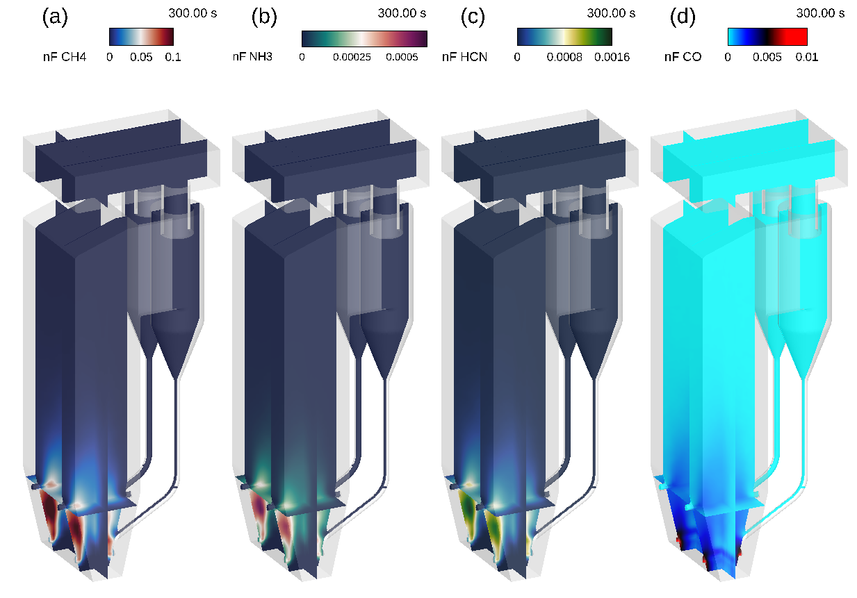
In the fluid phase, Barracuda accurately captures the release and reaction of volatile species that primarily form CO2, as well as several less-desirable side products. Looking back at the previous animations in Figure 3c, the discrete mass fraction of volatiles was shown to drop to zero just as the coal was fed into the riser, indicating a rapid release of volatile species. Now in the fluid phase, the release of four key volatile species: methane (CH4), ammonia (NH3), hydrogen cyanide (HCN), and carbon monoxide (CO) is shown in Figure 4. The Figure 4 animations focus on the space near the coal inlets of the CFB. Each of the above-mentioned volatiles is shown to be present just above the coal inlets, supporting the quick devolatilization shown in Figure 3c. These released species then react away quickly and are not present in appreciable quantities above the four secondary air inlets. This becomes more apparent when viewing the same results averaged over 150 seconds (Figure 5). A distinct profile, shared by each volatile species shown in Figure 4, is observed, showing higher concentrations in the space between the coal and secondary air inlets on both sides of the riser.
Figure 4a: Fluid Domain Mole Fraction CH4, 4b: Fluid Domain Mole Fraction NH3, 4c: Fluid Domain Mole Fraction HCN, 4d: Fluid Domain Mole Fraction CO
The volatile release is followed by a series of reactions primarily producing CO2 and H2O, with NO as a key side product to be limited. Oxygen is needed for each of these reactions to occur, and is supplied primarily through the fluidizing air inlet at the bottom of the riser. Refer to the animation in Figure 6, where instantaneous gas phase mole fractions are shown across slices in the z and y planes at the locations of the coal and secondary air inlets. In Figure 6a, a high concentration of oxygen exists just above the primary air inlet, and the concentration decreases quickly with elevation. Another couple of feet above, and the oxygen concentration falls to within 3% mole fraction. Oxygen is consumed quickly in the riser and reacts exothermically to form CO2. In Figure 6b, CO2 is observed forming in areas where oxygen is consumed. The highest concentration of CO2 exists in the transition zone above the primary air inlet and between the secondary air inlets. The time-averaged concentrations in Figure 7 better illustrate the higher CO2 concentrations in this transition zone, while the instantaneous view provides insight into the system’s dynamic nature.
Several byproducts form in the CFB and must be minimized to reduce the harmful environmental impacts of their release into the atmosphere. NO is a key combustion product and a pollutant formed here. In Figure 6c, the distribution of NO throughout the system is shown. NO forms in CFBs by oxidizing released nitrogenous volatile species (NH3 and HCN, for example); therefore, the dense zone must be kept as fuel-rich and relatively oxygen-poor to ensure that too much NO does not form. The instantaneous and time-averaged animations of oxygen distribution show that, while large volumes of primary air are supplied to the system, it is consumed very quickly, limiting the potential for NO formation in the dense bed. The dense bed NO reacts with carbon char on the surface of coal fed to the riser and also participates in oxidation reactions with nitrogenous volatile compounds, leading to a decrease in NO concentration with elevation. Water vapor (H2O(v) in Figure 6d) is formed in the dense portion of the riser either as a volatile itself or through reactions between volatile species. The highest concentrations of H2O(v) in the system are located around the coal inlets, indicating that the ammonia and hydrogen cyanide released as volatiles react with the primary air in these regions. Further up the riser, we see a sharp decline in NO concentrations around the secondary air inlets, along with a trail of high-concentration steam in the same area. The reaction of NO with volatiles and oxygen supplied by the secondary air inlets produces steam, which explains the drop-off in NO concentration near the secondary air inlets.
Figure 6a: Fluid Domain Mole Fraction O2, 6b: Fluid Domain Mole Fraction CO2, 6c: Fluid Domain Mole Fraction NO, Fluid Domain Mole Fraction H2O
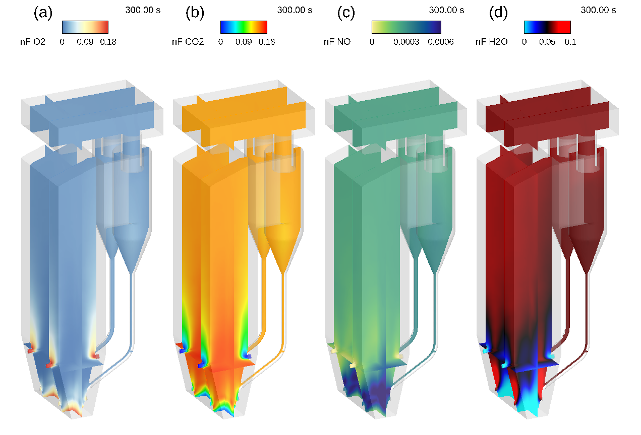
Figure 7a: Time-Averaged Mole Fraction O2, 7b: Time-Averaged Mole Fraction CO2, 7c: Time-Averaged Mole Fraction NO, 7d: Time-Averaged Mole Fraction H2O
Heat transfer within the system occurs quickly, as particles fed into the riser achieve a temperature rise from 200 K to 1400 K in seconds. Figure 8 shows animations of particle and fluid temperatures. Figure 8a shows the rapid heating and circulation of coal particles throughout the system. Heating occurs rapidly due to exothermic reactions in the riser and the 60,000 kilograms of ash circulating through the system, which serves as an excellent heat-transfer agent. In this model, the heat capacities of coal, ash, and all fluid species are functions of temperature. The right-most animation in Figure 8b provides insight into the predicted fluid temperatures in the CFB. The centerline temperature in the riser is predicted to be around 1200 K, with the incoming secondary and primary air heating rapidly due to reactions and heat transfer from high-solids circulation.
Figure 8a: Coal Particle Temperature over Time (K), 8b: Fluid Domain Temperature (K)
Modeling Instructions
Circulating Fluidized Bed (CFB) Combustor Simulation Setup
The user is expected to have already completed the basic Barracuda training, Barracuda Virtual Reactor New User Training (cpfd-software.com).
-
- Download the Industrial CFB Combustor Support File from this link.
- Unzip the support file and place it in the working directory set up for this CFB project.
- Open a new Barracuda session.
- From the File menu, choose Open Project. Navigate to the working directory and select CFB.prj.
-
The project file has already been set up with the appropriate.prj
-
- Grid.
- Base Materials.
- Particles.
- Initial Conditions
-
- Fluid ICs.
- Particle Species.
-
- Boundary Conditions
-
- Pressure BCs.
- Flow BCs.
-
- Chemistry
The chemistry setup for this project, which is already complete, is described in detail below.
Chemistry
Rate Coefficients
Many of the rate coefficients in the kinetic model (such as k0) follow the standard Arrhenius form, requiring only a pre-exponential factor (C0) and an activation energy to be specified. Several rate constants include a particle-dependence specification, resulting in the overall rate being influenced by the total mass (k6), volume fraction (k35), diameter (k35), or area (k13) of a specific species. A common inclusion in the kinetics is a term that accounts for the volume of fluid present in a given control volume (θf). The instructions below describe the setup of the rate constant k9, which encompasses all of the previously described parameters.
-
- Under Chemistry, select Rate Coefficients. Click Add to bring up the Chemistry Coefficient Editor. Volume-Average, which is the default reaction type, is used for this rate constant.
- Add the following equation parameters shown in Figure 11.
-
- Enter a value of 0.0005218 for C0, the pre-exponential factor.
- Enter a value of 2 for C1 to account for the second-order temperature value (T2).
- Enter a value of 1 for C4 to account for the volume of fluid present, θf.
- Specify an activation energy of 6319 and an initial activation energy of -17.29.
- Select Particle Dependence in the Chemistry Coefficient Editor
-
- From the Project Materials List, add C to the Materials List, selecting mass for the Material Coefficient Type.
- Select a mass unit of kg/m3.
-
-
Entering the remaining rate constants follows a similar procedure, ensuring that the correct particle dependencies and parameters are accounted for in each equation. All of the rate constant equations are intended for volume average chemistry, apart from k30 and k28, which are to be used for discrete rate expressions. Discrete reactions must be specified differently and refer to heterogeneous reactions occurring directly on the particle surface, whereas volume-average chemistry concerns homogeneous reactions. Two of the rate constant expressions are user-defined (k12 and k28), and their expressions are shown below in Figures 9 and 10.
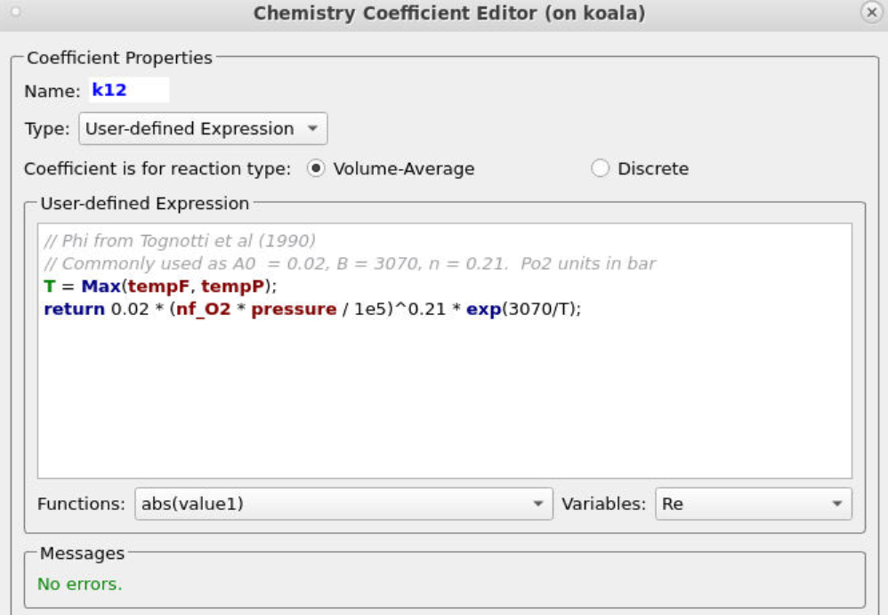
Figure 9: User-Defined Expression for k12
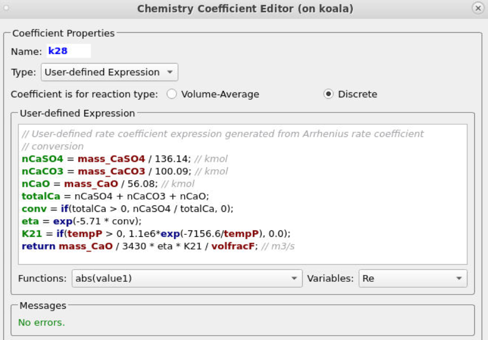
Figure 10: User-Defined Expression for k28
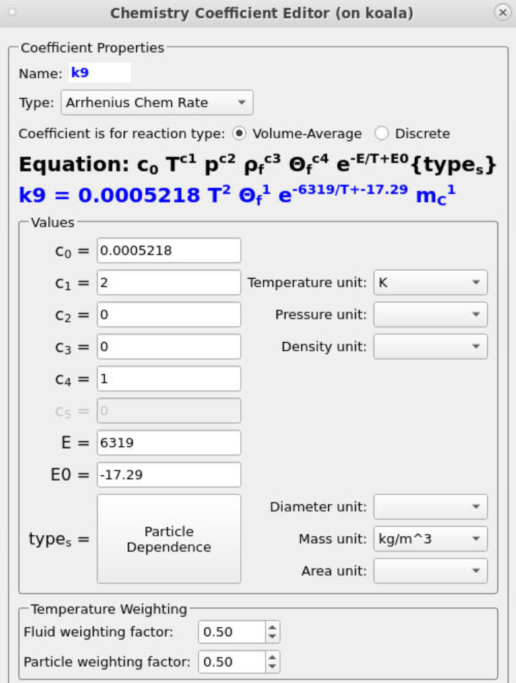
Figure 11: Arrhenius Expression for k9
Reactions
The reaction set included in this kinetic model comprises 29 reactions. 27 of these reactions occur in the fluid phase and follow homogeneous-volume-average chemistry. The procedure for entering reactions in Barracuda is shown below, using reaction 1 and rate expression 0 as examples.
-
- Under Chemistry, select Reactions. Click Add ⇒ Volume-Average: Stochiometric rate equation to bring up the Chemistry Stochiometric Equation Editor.
-
- Under Equations Units, select mol/m3/sec for Reaction rate units and mol/m3 for Fluid species units.
- Enter the Stoichiometric reaction for water gas shift as shown in Figure 8.
- Enter the rate equation R0 for the stoichiometric reaction as shown in the box R00.
- Click OK to close the Chemistry Stochiometric Equation Editor.
-
- Under Chemistry, select Reactions. Click Add ⇒ Volume-Average: Stochiometric rate equation to bring up the Chemistry Stochiometric Equation Editor.
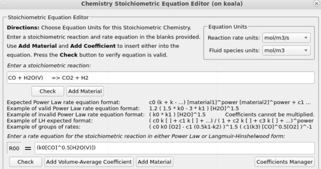
Figure 12: Water Gas Shift Reaction Stoichiometry
The two discrete reactions must be specified differently. The first discrete reaction, shown in Figure 13, specifies the rates at which volatile species are to be released from the coal fed into the system. The rate is the mass of volatiles released per unit time, expressed in kg/s. The rates at which each species is released are calculated from the coal species composition and are crucial for determining accurate compositions throughout the system. The CaO in the ash can absorb some of the SO2 as calcium sulfate (CaSO4); this discrete reaction is shown in Figure 14.
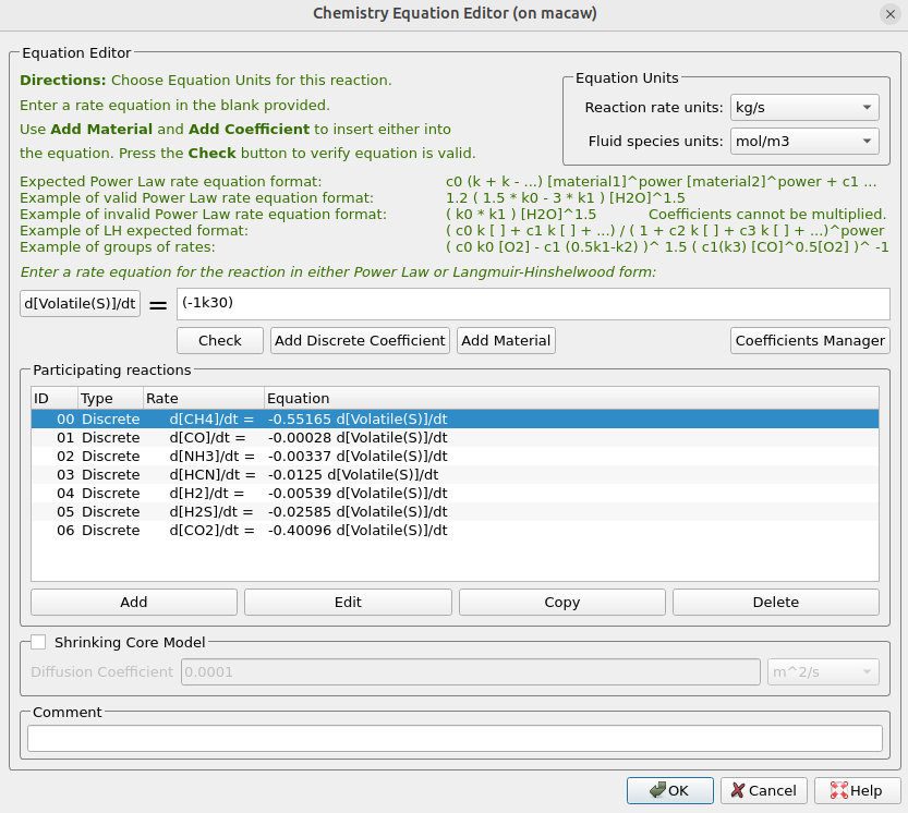
Figure 13: Volatile Release
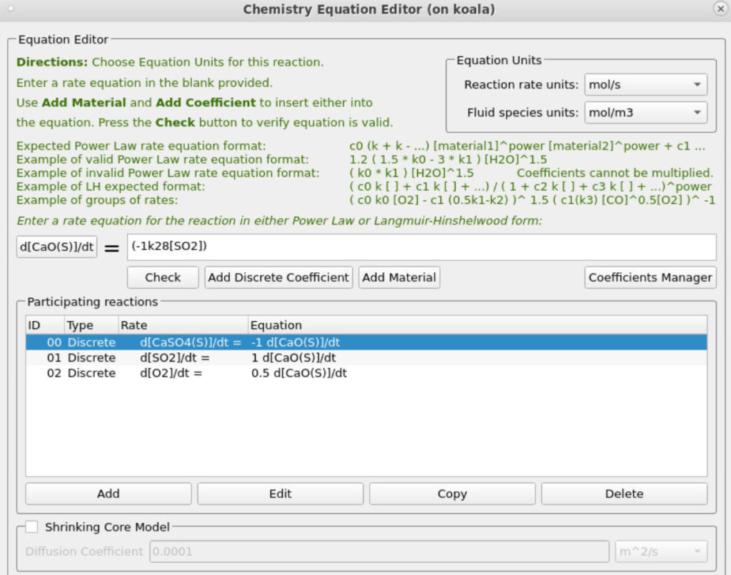
Figure 14: SO2 Release
Time Controls
-
- Enter 1.5e-4 secs for Time Step and 300 seconds for End Time.
- Put 0.1 secs for the Restart Interval.
Visualization Data
-
- Enter 0.2 secs for the Output file interval.
- Select the Visualization Data for post-processing as shown in Figure 15.
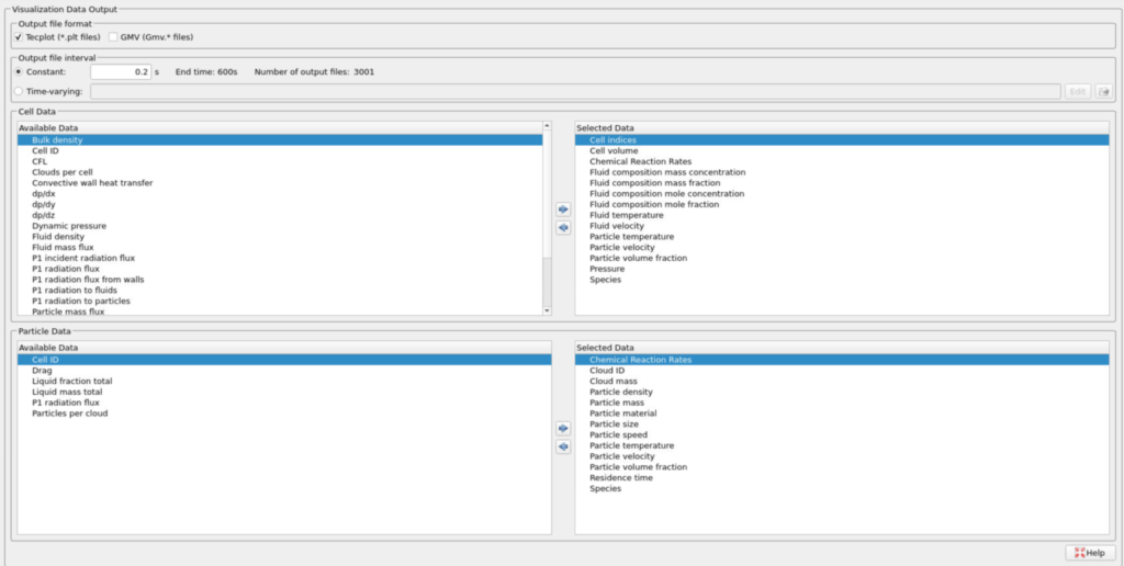
Figure 15: Selected Visualization Data for CFB Combustor Model
Run
-
- Click on Run and then click on Run Solver.
- Select GPU Parallel if you have the required GPU parallel license.
Post-Processing CFB Combustor Results in Tecplot
The user is assumed to have gone through basic Tecplot training, Getting Started With Tecplot For Barracuda® | CPFD Software (cpfd-software.com), and the training material in “Tecplot for Barracuda – Using frames” (Tecplot for Barracuda – Using Frames | CPFD Software (cpfd-software.com)). Only a few brief steps for post-processing the results are explained.
To recreate the images and animations of Figures 3 – 8, use the layout (.lay) files held within the support file provided in the Circulating Fluidized Bed (CFB) Combustor Simulation Setup section of this post. Refer to the instructions below to load them in Tecplot for Barracuda.
-
- In the Barracuda GUI window, navigate down to Post-Run in the project tree, and select the View Results tab.
- In the resulting Tecplot window, select File, then Open Layout, and select from your file system one of the provided 6 layout files.
This concludes the description of the simulation setup process for Application Model: Circulating Fluidized Bed Combustor.
References
-
- Krusch, S. (2018). Experimental examination and simulation of a pilot-scale circulating fluidized bed reactor (Doctoral dissertation, Ruhr University Bochum). Ruhr-Universität Bochum.
-
Lyon, R. K., Hardy, J. E., & Von Holt, W. (1985). Oxidation kinetics of wet CO in trace concentrations. Combustion and Flame, 59(1), 45–60. https://doi.org/10.1016/0010-2180(85)90074-4
- Lockwood, Toby. Techno-economic Analysis of PC versus CFB Combustion Technology. IEA Clean Coal Centre, Oct. 2013, ISBN 978-92-9029-546-4.
-
Silcox, G. D., Kramlich, J. C., & Pershing, D. W. (1989). A mathematical model for the flash calcination of dispersed CaCO₃ and Ca(OH)₂ particles. Industrial & Engineering Chemistry Research, 28(2), 155–160. https://doi.org/10.1021/ie00086a005
-
Tighe, C. J., Twigg, M. V., Hayhurst, A. N., & Dennis, J. S. (2012). The kinetics of oxidation of Diesel soots by NO₂. Combustion and Flame, 159(1), 77–90. https://doi.org/10.1016/j.combustflame.2011.06.009
-
Wu, Y., Liu, D., Ma, J., & Chen, X. (2017). Three-dimensional Eulerian–Eulerian simulation of coal combustion under air atmosphere in a circulating fluidized bed combustor. Energy & Fuels, 31(8), 7952–7966. https://doi.org/10.1021/acs.energyfuels.7b00762
-
Xie, J., Zhong, W., Jin, B., Shao, Y., & Liu, H. (2014). Three-dimensional Eulerian–Eulerian modeling of gaseous pollutant emissions from circulating fluidized-bed combustors. Energy & Fuels, 28(8), 5523–5533. https://doi.org/10.1021/ef501095r
-
Xie, J., Zhong, W., Shao, Y., Liu, Q., Liu, L., & Liu, G. (2017). Simulation of combustion of municipal solid waste and coal in an industrial-scale circulating fluidized bed boiler. Energy & Fuels, 31(12), 14248–14261. https://doi.org/10.1021/acs.energyfuels.7b02693
- Yang, Miao, et al. “CFD Simulation of Biomass Combustion in an Industrial Circulating Fluidized Bed Furnace.” Combustion Science and Technology, vol. 195, no. 14, 2023, pp. 3310–3340, Taylor & Francis, doi:10.1080/00102202.2023.2260553.