
Introduction
Fossil fuels usage accounts for 96% of the 60 million tons of hydrogen (H2) produced world wide (Al-Qahtani’ 2020). Currently steam methane reforming combined with carbon capture and storage is the lowest-total cost hydrogen production method (Al-Qahtani’ 2020). One such pre-combustion carbon capture technology is sorbent enhanced steam methane reforming (SE-SMR), which integrates both H2 production and CO2 capture.
This application model exemplifies the usage of compressible isothermal flow setup with both volumetric and discrete reaction chemistry in Barracuda Virtual Reactor (referred to as Barracuda in rest of this application model post). Two simulation setups are shown in this application model. First the SE-SMR model setup is shown in Barracuda. Then the SE-SMR model setup is converted into steam methane reforming (SMR) model setup allowing for comparison of CO2 capture between the two processes.
Model Definition
The reactor geometry modeled in this application is sourced from the work of Wang et. al’ 2022. Figure 1 shows the reactor model geometry, 100 mm in diameter and 1000 mm in height. The catalyst used in the simulation is Nickel based. Calcined Dolomite is used as the sorbent. The catalyst-to sorbent mass ratio is 2.44. The reactor wall is at fixed temperature of 873.15 K and the initial catalyst bed height in the reactor is set to 300mm. Steam and methane, with a molar ratio of 3, are injected from the bottom Flow BC at a velocity of 0.032 m/sec to fluidize bed. The top boundary is defined as a pressure BC at atmospheric pressure.
The Ni-catalyst particle sizes are between 150-250 microns, whereas Dolomite particle sizes are between 125-300 microns. WenYu-Ergun drag model is used for both the particle species. The material properties of the gases and solid particles are a function of temperature in this simulation. All gases are assumed to show ideal gas behavior.
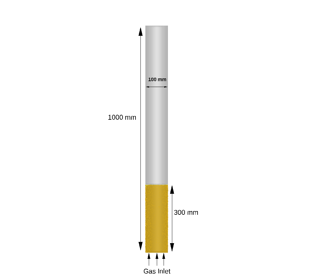
Figure 1: Bubbling Fluidized Bed SE-SMR and SMR Reactor Domain.
Reaction Kinetics
In steam methane reforming process the majority of CH4 is converted into CO2 and H2 through global reversible reactions including two steam methane reforming reactions and a water-gas shift reaction as shown below.
$$ SMR: CH_4 + H_2O \iff CO +3H_2 $$
$$ SMR: CH_4 + 2H_2O \iff CO_2 +4H_2 $$
$$ WGS: CO + H_2O \iff CO_2 + H_2 $$
The SE-SMR process includes an additional carbonation reaction for sorbent capture of CO2 ,
$$ CaO + CO_2 \iff CaCO_3 $$
The reaction kinetics for reforming and water-gas shift reactions taken from Xu and Froment’ 1989 are shown below,
\begin{align}
R_1 &= \frac{k_1}{p_{H_2}^{2.5} (DEN)^2} \left(P_{CH_4} P_{H_2 O} – \frac{P_{H_2}^3 P_{CO}}{K_{\mathrm{I}}} \right) \\
R_2 &= \frac{k_2}{p_{H_2}^{3.5} (DEN)^2} \left(P_{CH_4} P_{H_2 O}^2 – \frac{P_{H_2}^4 P_{CO_2}}{K_{\mathrm{II}}} \right) \\
R_3 &= \frac{k_3}{p_{H_2} (DEN)^2} \left(P_{CO} P_{H_2 O} – \frac{P_{H_2} P_{CO_2}}{K_{\mathrm{III}}} \right)
\end{align}
\begin{align}
DEN &= 1 + K_{CO} P_{CO} + K_{H_2} P_{H_2} + K_{CH_4}P_{CH_4} + \frac{K_{H_2 O} P_{H_2 O} }{P_{H_2}} \\
\end{align}
The rate coefficients for kinetic constants k1, k2 and k3 given by Xu and Froment’ 1989 are as follows,
\begin{align}
k_1 &= 1.842 \times 10^{-4} exp\left[\frac{-240100}{R} \left(\frac{1}{T} – \frac{1}{648}\right) \right] \ kmol \cdot bar^{0.5}/(kg_{cat} \cdot h) \\
k_2 &= 2.193 \times 10^{-5} exp\left[\frac{-243900}{R} \left(\frac{1}{T} – \frac{1}{648}\right) \right] \ kmol \cdot bar^{0.5}/(kg_{cat} \cdot h) \\
k_3 &= 7.558 exp\left[\frac{-67130}{R} \left(\frac{1}{T} – \frac{1}{648}\right) \right] \ kmol/(kg_{cat} \ h \cdot bar) \\
\end{align}
The equilibrium constants of reaction KI, KII and KIII given by Xiu et. al’ 2002 are as follows ,
\begin{align}
K_{\mathrm{I}} &= 4.707 \times 10^{12} exp\left(\frac{-224000}{RT} \right) bar^{2} \\
K_{\mathrm{II}} &= K_{\mathrm{I}} \cdot K_{\mathrm{III}} bar^{2} \\
K_{\mathrm{III}} &= 1.142 \times 10^{-2} exp\left(\frac{37300}{RT} \right) \\
\end{align}
The adsorption equilibrium constants KCH4, KH2O, KCO and KH2 given by Xu and Froment’ 1989 are as follows,
\begin{align}
K_{CH_4} &= 0.179 exp\left[\frac{38280}{R} \left(\frac{1}{T} – \frac{1}{823}\right) \right] bar^{-1} \\
K_{H_2 O} &= 0.4152 exp\left[\frac{-88680}{R} \left(\frac{1}{T} – \frac{1}{823}\right) \right] \\
K_{CO} &= 40.91 exp\left[\frac{70650}{R} \left(\frac{1}{T} – \frac{1}{648}\right) \right] bar^{-1} \\
K_{H_2} &= 0.00296 exp\left[\frac{82900}{R} \left(\frac{1}{T} – \frac{1}{648}\right) \right] bar^{-1} \\
\end{align}
The kinetics of carbonation taken from Sun et.al’ 2008 are shown below,
\begin{align}
r_{carb} &= k_{carb} \left(p_{CO_2} – p_{CO_{2,eq}}\right)^n S_0 \left(1 – X_{CaO}\right) \\
\end{align}
The equilibrium pressure of CO2 is dependent on ranges of temperatures as follows:
For T > 1173.5 K
\begin{align}
p_{CO_2, eq} &=1.216 \times 10^{12} exp\left(\frac{-19130}{T} \right) \\
\end{align}
For T<= 1173.5 K
\begin{align}
p_{CO_2, eq} &=4.1918 \times 10^{12} exp\left(\frac{-20474}{T} \right) \\
\end{align}
Rate constants of carbonation (kcarb) and degree of partial pressure (n) are dependent on PCO2 ranges as follows
for \(\left(p_{CO_2} – p_{CO_2,eq} \right)\) > 10,000 pa:
\begin{align}
k_{carb} &=1.04\times 10^{-6} exp\left(\frac{-20400}{RT} \right) kmol \cdot m^{-2} \cdot s^{-1} \\
n = 0 \\
\end{align}
for 0 < \(\left(p_{CO_2} – p_{CO_2,eq} \right)\) <= 10,000 pa:
\begin{align}
k_{carb} &=1.04\times 10^{-10} exp\left(\frac{-20400}{RT} \right) kmol \cdot m^{-2} \cdot Pa^{-1} \cdot s^{-1} \\
n = 1\\
\end{align}
for \(\left(p_{CO_2} – p_{CO_2,eq} \right)\) <= 0 pa, no CO2 is captured i.e. decarbonation occurs instead.
Results and Discussion
Figure 2 shows the Barracuda simulation predicted CO2 mole fraction in the bubbling fluidized bed reactor domain for SE-SMR and SMR cases. In the SE-SMR process, the CO2 produced from the steam methane reforming and water gas shift reactions is absorbed by the dolomite particles as we move further away from the inlet of the reactor, resulting in negligible amounts of CO2 leaving the reactor from the top boundary. On the other hand, in the SMR process, the produced CO2 leaves the reactor. To avoid greenhouse gas emissions this produced CO2 from the SMR process needs to be captured using post-combustion technologies which increases the cost of the H2 production.
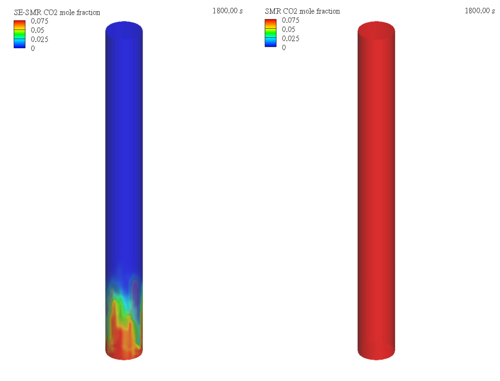
Figure 2: CO2 mole fraction. Sorbent-enhanced Steam Methane Reforming (left); Steam Methane Reforming (Right)
Modeling Instructions
Sorbent-Enhanced Steam Methane Reforming (SE-SMR) Reactor Simulation Setup
The user is expected to have already gone through basic Barracuda training Barracuda Virtual Reactor New User Training | CPFD Software (cpfd-software.com).
- Download the support files provided along with this post.
- Unzip the support file and place it in the working directory setup for this SE-SMR project.
- Open a new Barracuda session.
- From the File menu, choose Open Project. Navigate to the working directory and select SE_SMR.prj.
The project file has already been setup with the appropriate
- Grid.
- Base Materials.
- Particles.
- Initial Conditions
- Fluid ICs.
- Particle Species.
- Boundary Conditions
- Pressure BCs.
- Flow Bcs.
The chemistry setup for this project, which is already setup, is described in detail below.
Chemistry
Rate Coefficients
The reaction kinetics described above need to be converted into a format that is acceptable for inputting into Barracuda.
- Under Chemistry, select Rate Coefficients. Click Add to bring up the Chemistry Coefficient Editor. Volume-Average, which is the default reaction type, is used for kinetic constants k1, k2, and k3, equilibrium constants of reaction KI, KII, and KIII, and the adsorption equilibrium constants KCH4, KH2O, KCO, and KH2.
- Reaction kinetic constant k1 will be first input into Barracuda. The units of k1 are kmol bar0.5/kgcat ·hr these need to be converted to kmol bar0.5/m3 ·sec in the Chemistry Coefficient Editor as shown in the following steps.
- Divide k1 by 3600 to convert the units to per second.
- Divide 1.842×10-4 by 3600 and input the value as CO in the Chemistry Coefficient Editor. Leave Type set to Arrhenius Chem Rate.
- Click on Particle dependence in the Chemistry Coefficient Editor.
- In the Particle dependence window, from the Project Materials List, add Ni to the Materials List. For the Material coefficient type, select mass.
- Click OK to close the Particle dependence window.
- Select Mass unit as kg/m3 in the Chemistry Coefficient Editor.
- Divide k1 by θf. Where θf is the volume of fluid in a given control volume.
- To do this, put -1 in for C4 in the Chemistry Coefficient Editor.
- The values in the exponential in k1 are multiplied through and divided by the Universal gas constant R = 8.314 KJ/Kmol ·K.
- Enter 28879 for E.
- Enter 44.567 for E0.
- Optional: Add units kmol bar0.5/m3 ·sec in the comment box.
- Divide k1 by 3600 to convert the units to per second.
- Reaction Kinetic constant k2 and k3 can be entered in the same way, following the steps given above for k1.
- The equilibrium constants of reaction KI, KII, and KIII are in an acceptable format for inputting into Barracuda and can be entered directly.
- Notethat the KII is a product of KI and KIII.
- The adsorption equilibrium constants KCH4, KH2O, KCO, and KH2 are also in an acceptable format for inputting into Barracuda and can be entered directly.
- Reaction kinetic constant k1 will be first input into Barracuda. The units of k1 are kmol bar0.5/kgcat ·hr these need to be converted to kmol bar0.5/m3 ·sec in the Chemistry Coefficient Editor as shown in the following steps.
- In SE-SMR process the carbonation reaction involving the dolomite particles is a discrete reaction. Therefore this will be defined as such in Barracuda.
-
- Click Add to bring up the Chemistry Coefficient Editor. Change the reaction type to Discrete. From the drop down list under Type select User-defined Expression.
-
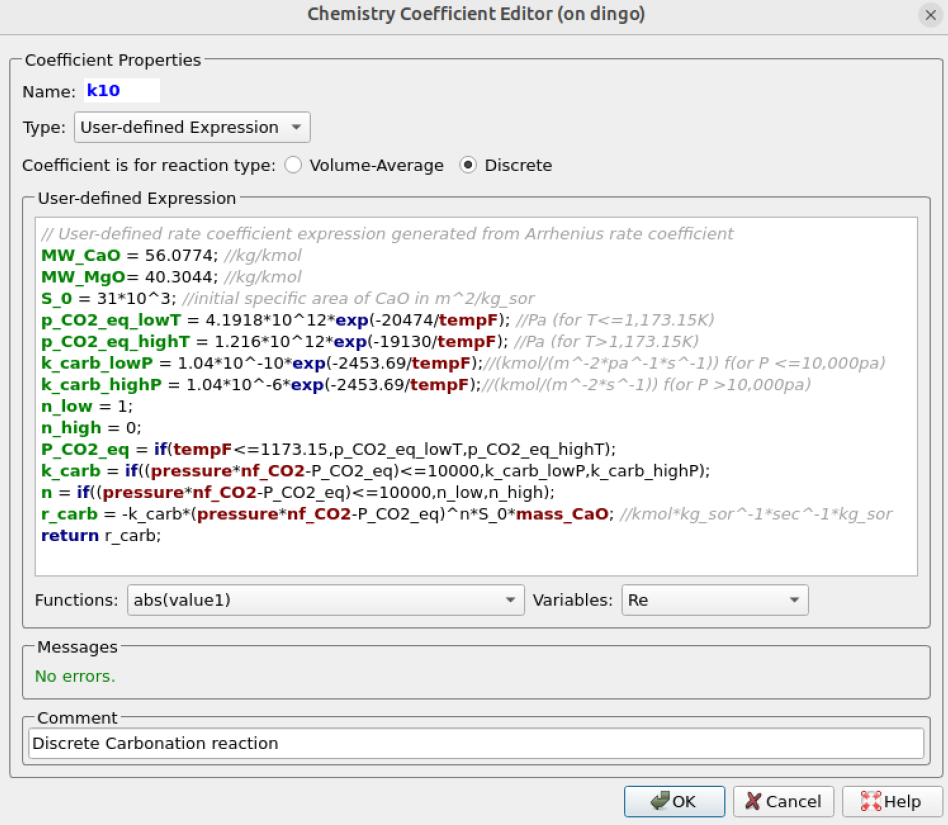
Figure 3: Discrete Carbonation Reaction Kinetics for SE-SMR Reactor Simulation.
Figure 3 shows a screenshot of the Discrete carbonation reaction kinetics setup in Barracuda for the SE-SMR process.
- Replicate the discrete reaction kinetic, rcarb, setup as shown in Figure 3. A few key points to note are:
- The initial specific surface area (S_0) value is taken from Johnsen et. al’ 2006.
- The mathematical exponent function, exp, as well as logical function, IF, used in figure 3 are obtained from the drop down list under Functions.
- To enter a function in the User-defined Expression editor place the cursor at the desired location and select the function needed from the drop down list.
- The variables such as tempF, pressure nf_CO2, and mass_CaO are obtained from the drop-down list under Variables.
- To enter a variable in the User-defined Expression editor place the cursor at the desired location and select the variable needed from the drop down list.
- The reaction rate for gas-solid reaction is defined as a specific rate, where r_{carb} = dX/dt cdot (1-X). The derivative for “X” is taken while entering the expression for rcarb.
Reactions
To finish setting up the chemistry portion of this simulation, the methanation, water-gas shift, and carbonation reactions need to be entered into Barracuda.
- Under Chemistry, select Reactions. Click Add ⇒ Volume-Average: Stochiometric rate equation to bring up the Chemistry Stochiometric Equation Editor.
- Under Equations Unit,s select kmol/m3/sec for Reaction rate units and bar for Fluid species units.
- Enter the Stoichiometric reaction for methane reforming as shown in Figure 4.
- Enter the rate equation R1 for the stoichiometric reaction as shown in the box R00.
- Click OK to close the Chemistry Stochiometric Equation Editor.
- Repeat steps 1 to 4 and enter all the remaining SMR and WSG reactions.
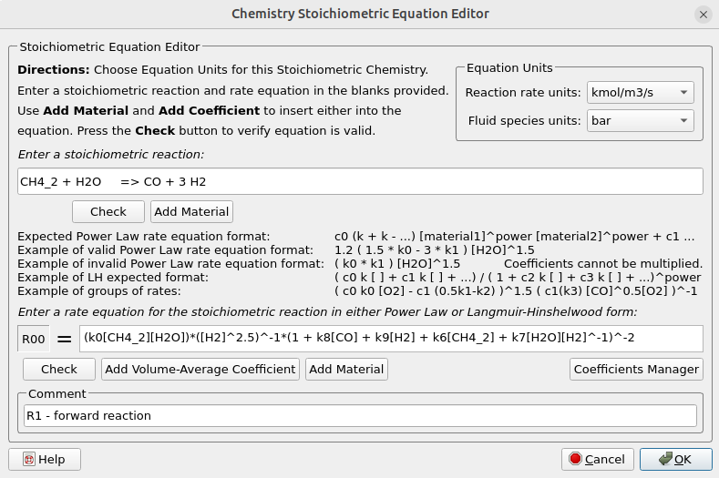
Figure 4: Volume-average Stochiometric Reactions and Rate Equations for SE-SMR Reactor Simulation.
- Under Chemistry select Reactions. Click Add ⇒ Discrete: Particle rate equation to bring up the Chemistry Equation Editor.
- Under Equations Units select kmol/sec for Reaction rate units and kg/m3 for Fluid species units.
- Enter the rate equation for carbonation as shown in figure 5.
- Click on Select Species and pick CaO(S) from the Chemistry Materials Selection box.
- Enter the Participating reactions as shown in figure 5.
- Click OK to close the Chemistry Equation Editor.
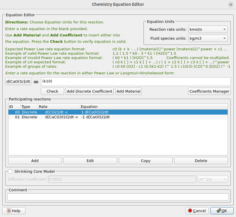
Figure 5: Discrete Reaction and Rate Equation for SE-SMR Reactor Simulation.
Time Controls
- Enter 5e-4 secs for Time Step and 1800 secs for End Time.
- Put 100 secs for the Restart Interval.
Visualization Data
- Enter 60 secs for Output file interval.
- Select the Visualization Data for post processing as shown in Figure 6.
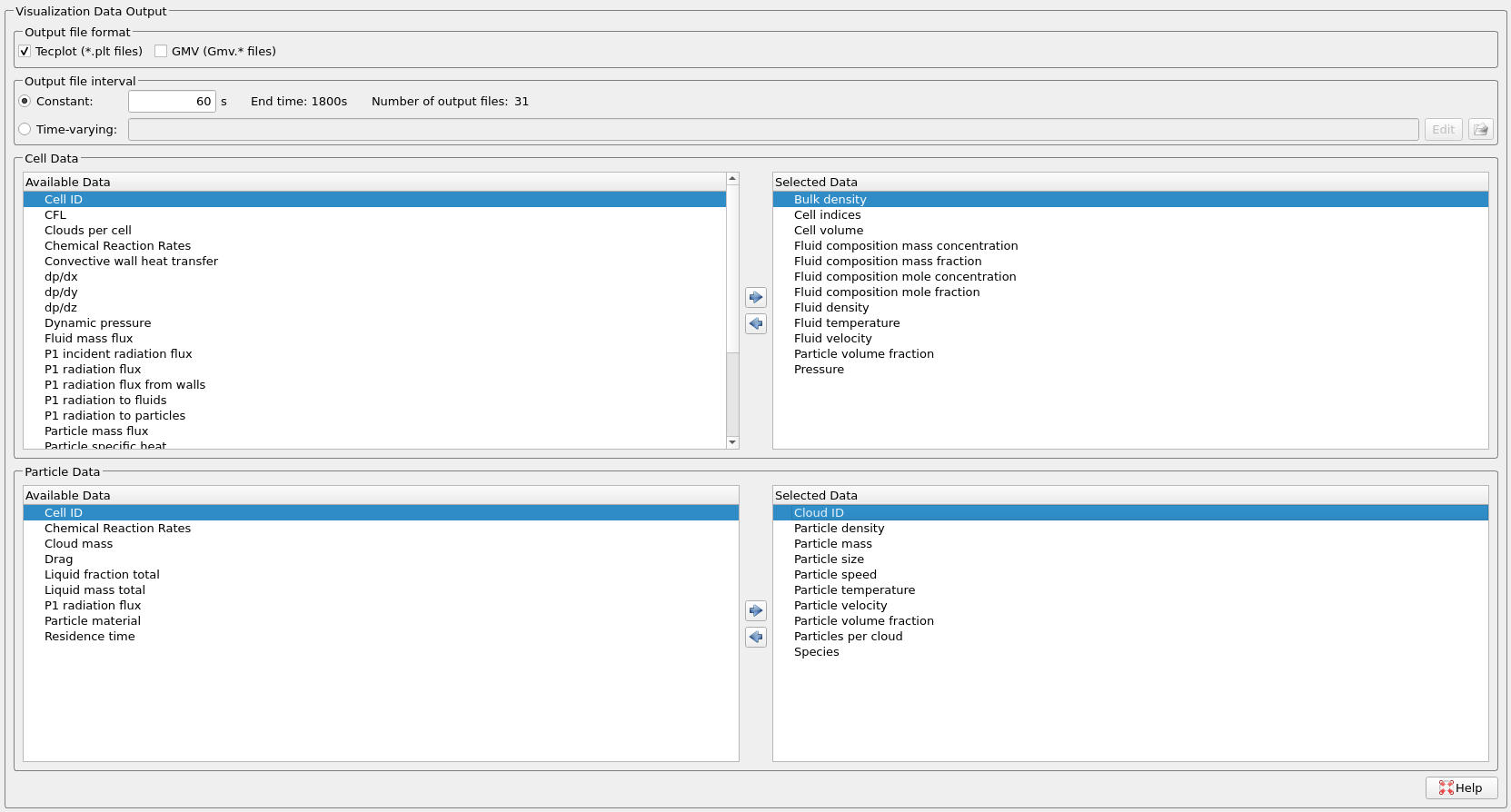
Figure 6: Visualization Data selected for SE-SMR Reactor Simulation.
Run
- Click on Run and then click on Run Solver.
- Select GPU Parallel if you have the required GPU parallel license.
Post Processing SE-SMR Results in Tecplot
The user is assumed to have gone through basic Tecplot training, Getting Started With Tecplot For Barracuda® | CPFD Software (cpfd-software.com). So, only a few brief steps for post-processing the results are explained.
- In the Barracuda GUI, click on Post-Run and then click on View Results.
- Deselect Scatter from the Plot menu.
- Check Contour Box
- Click on settings beside Contour to open up the Contour & Multi-Coloring Details window.
- From the drop-down list, select Fluid domain mole fraction CO2(G).
- From the drop-down list under Color map options, select Modified Rainbow – Less Green.
- Click on Set Levels and set the Minimum level to 0, Maximum level to 0.075, and Number of levels to 4.
- Under the Color map distribution method, change the method to Continuous.
- For contour values at end points, enter 0 for Min and 0.075 for Max.
- Click on the Close button to close the Contour & Multi-Coloring Details window.
Steam Methane Reforming (SMR) Reactor Simulation Setup
The existing SE-SMR reactor simulation setup can be converted into a SMR reactor simulation setup as shown below.
- From the File menu, choose Save Case As. Save the project file as SMR.prj in a different newly created directory.
- Go to the Chemistry Reactions Manager window and delete the discrete reaction.
- Go to the Chemistry Rate Coefficients Manager window and delete the Discrete Rate Coefficient (k10).
- Go to Particle IC Manager and delete the dolomite species (ID = 001).
- Go to Particles Species Manager, delete dolomite species (Species-ID = 002).
- Finally, go to Base Materials and delete CaO and MgO from the Project Material List.
- Click on Run and then click on Run Solver.
Adding SMR results to SE-SMR Results in Tecplot
To create the contour plot shown in Figure 2, follow the steps shown below.
- Tecplot frames are used to add SMR results to the existing SE-SMR results in the open Tecplot instance. The user is expected to have already gone through the training material in “Tecplot for Barracuda – Using frames” (Tecplot for Barracuda – Using Frames | CPFD Software (cpfd-software.com)).
- From the top menu bar in Tecplot, select Frame ⇒ Create New Frame.
- Select Tile frames from Frame and tile the frames vertically.
- Select Frame ⇒ Frame Linking, and then check the boxes for Solution Time, 3D plot view.
- Go to File and select Load Barracuda data ,and then select Load 3D dataset.
- Go to the working directory for SMR simulation and select bvr.cells.0000.plt.
- Follow the main steps 1 to 4 shown in in Post Processing SE-SMR Results in Tecplot section to create a contour plot for CO2 mass fraction.
This concludes the description of the simulation setup process for Application Model: Hydrogen Production with Sorbent Enhanced Steam Methane Reforming (SE-SMR) in Barracuda Virtual Reactor.
References
Wan, Z., Yang, S., Bao, G., Hu, J., & Wang, H. (2022). Multiphase particle-in-cell simulation study of sorption enhanced steam methane reforming process in a bubbling fluidized bed reactor. Chemical Engineering Journal, 429, 132461.
Xu, J., & Froment, G. F. (1989). Methane steam reforming, methanation and water‐gas shift: I. Intrinsic kinetics. AIChE journal, 35(1), 88-96.
Xiu, G. H., Li, P., & Rodrigues, A. E. (2002). Sorption-enhanced reaction process with reactive regeneration. Chemical engineering science, 57(18), 3893-3908.
Sun, P., Grace, J. R., Lim, C. J., & Anthony, E. J. (2008). Determination of intrinsic rate constants of the CaO–CO2 reaction. Chemical Engineering Science, 63(1), 47-56.