
Introduction
Surface erosion due to solid particle impact, also known as solid particle erosion, is a complex, progressive process of material removal from a surface caused by the repeated impact of solid particles. This phenomenon occurs when hard particles, typically carried by a fluid medium (liquid or gas), collide with a solid surface at varying velocities and angles. Material erosion in industrial equipment such as gas cyclones, circulating fluidized bed boilers, etc., can often lead to performance reduction, reduced operational lifetime, and in some extreme cases, catastrophic equipment failure. While the amount of material removed from a surface during a solid particle impact is dependent on several variables, it can be broadly classified under ductile and brittle material behavior. In ductile materials, material erosion happens by a repeated cutting action of the impacting particle, causing plastic deformation of the eroding surface. On the other hand, in brittle material, erosion is driven by material cracking or fracturing and its subsequent propagation from the point of impact.
Key Parameters for Erosion Prediction
Several flow and material parameters influence erosion. Most of the erosion rate equations proposed in the literature have variables that can be broadly broken down into three types:
• Solid particle properties such as size, density, hardness, and shape have a significant influence on solid particle erosion.
• Particle impingement information, such as impact velocity of particles, impact angles, and particle-particle interaction (e.g., particle shielding in high solid loading flows), is closely tied with carrier fluid and flow properties. The characteristics of the carrier fluid, such as viscosity, density, and turbulent fluctuations, have a direct influence on particle trajectories, particle concentration, among other influences.
• Target surface material characteristics such as density, material hardness, and material mechanical properties such as Young’s and Poisson’s Modulus.
This application model demonstrates erosion prediction in a 90-degree elbow geometry using the Oka erosion model (Oka et. al’ 2005) available in Barracuda Virtual Reactor (referred to as Barracuda in the rest of this application model post).
Model Definition
The elbow model geometry modeled in this application is sourced from the work of Duarte et. al’ 2015. Figure 1 shows the 90-degree Aluminium elbow geometry with a diameter of 0.0254 m. A grid of 500,000 cells is used to set up the model. Sand particles are injected along with air at a velocity of 34.1 m/ sec into the elbow domain. Results from two different sand mass loading cases, namely 0.013 and 1.5, are shown in this application model post. Mass loading is defined as the ratio of kg of sand particles to kg of air injected. The flow is isothermal and compressible. The outlet boundary is defined as a pressure BC at atmospheric pressure. The average sand particle size is 182 microns. WenYu-Ergun drag model is used for the particle species. Air is assumed to show ideal gas behavior.
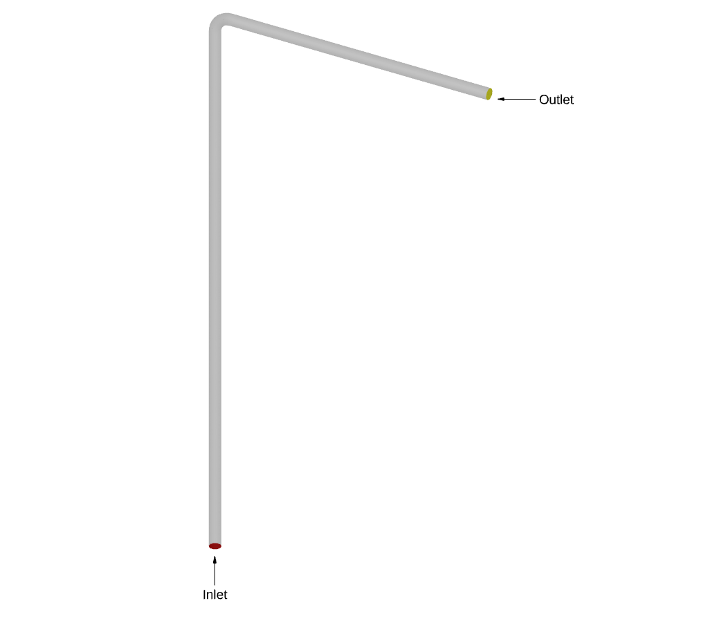
Figure 1: Elbow domain
Results and Discussion
Figure 2 shows the erosion pattern predicted by the Barracuda simulation for a mass loading of 0.013. The penetration ratio, which is defined as the thickness of material removed from the wall based on the mass of sand injected into the elbow, is shown. In Barracuda, the default units for the particle impacts resulting in wall erosion are kg/m2 /year. These units are converted into units of penetration ratio, m/kg. This unit conversion is discussed in detail in the post-processing section below in the post. The two-tail erosion pattern observed in the Barracuda simulation is similar to the erosion pattern observed in Duarte et. al’ 2015 at the same mass loading using one-way coupling.
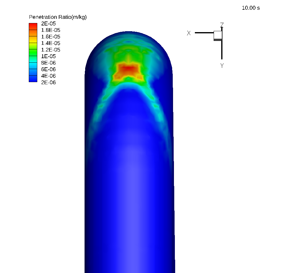
Figure 2: Erosion contours for mass loading of 0.013.
Figure 3 shows the penetration ratio (Y-axis) plotted as a function of curvature angle (X-axis) for mass loading 0.013. The curvature angle represents the bend in the elbow where erosion is analyzed. 0 degrees is the location of the bend closer to the inlet, while 90 degrees represents the end of the bend, closer to the outlet. The solid black line represents the results from Barracuda, and the black “+” symbol represents the simulation results from Duarte et. al’ 2015. The experimental results from the work of Mazumder et. al’ 2008 are also plotted and are shown with blue filled circles (error bars are also shown for the experimental results). Good agreement is observed between the Barracuda simulation and the experimental results. Also, both the simulation results, the present work, and those of Duarte et.al’ 2015 are within the experimental uncertainty.
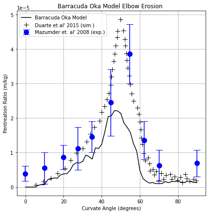
Figure 3: Penetration ratio plotted as a function of curvature angle for mass loading of 0.013.
To observe the effect of inter-particle collisions, a case with a higher mass loading of 1.5 was simulated in Barracuda. Figure 4 shows the erosion contours for mass loading of 1.5 with the particle collision model turned off (left) and with the particle collision model turned on (right). The results suggest that the inter-particle collisions protect the elbow surface from the direct impact of the incoming particles at the maximum penetration location. This is also known as the “cushioning effect”. This phenomenon is captured effectively by the Barracuda using the equilibrium and isotropy collision models. The usage of both these collisional models is demonstrated in detail later in this post. The two-tail erosion pattern prediction from the present Barracuda simulation, with the particle collision model turned off, Figure 4 (left), is in agreement with the erosion pattern prediction shown in Duarte’s one-way coupling higher mass loading case. Similarly, the converged tail erosion pattern prediction for the case with particle collision models turned on, Figure 4 (right), in Barracuda, is similar to Duarte’s four-way coupling for higher mass loading.
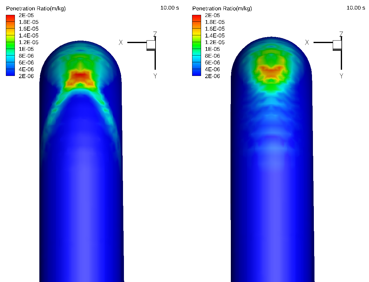
Figure 4: Erosion contours for mass loading of 1.5. Without particle collisions (left). With particle collisions (right).
Figure 5 shows the penetration ratio for the higher mass loading = 1.5 case with particle collision models turned on, plotted as a function of curvature angle (the legend of plots is the same as explained for Figure 4). Again, good agreement is observed between the present Barracuda simulation, the simulation results from Duarte et. al’ 2015, and the experimental results of Mazumder et. al’ 2008. Both the simulation results fall within experimental uncertainty.
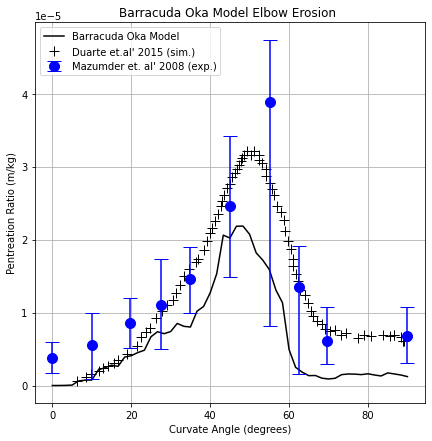
Figure 5: Penetration ratio plotted as a function of curvature angle for mass loading of 1.5.
Modeling Instructions
90-degree Elbow Erosion Simulation Setup
The user is expected to have already gone through basic Barracuda training Barracuda Virtual Reactor New User Training | CPFD Software (cpfd-software.com).
- Download the support files provided along with this post.
- Unzip the support file and place it in the working directory set up for this Erosion project.
- Open a new Barracuda session.
- From the File menu, choose Open Project. Navigate to the working directory and select erosion.prj.
The project file has already been set up with the appropriate
- Grid.
- Base Materials.
- Particles.
- Initial Conditions
- Fluid ICs.
- Particle Species.
- Boundary Conditions
- Pressure BCs.
- Flow BCs.
Time Controls
- Enter 1e-4 secs for Time Step and 10 secs for End Time.
- Put 100 secs for the Restart Interval.
Visualization Data
- Enter 0.5 secs for Output file interval.
- Select the Visualization Data for post processing as shown in Figure 6.
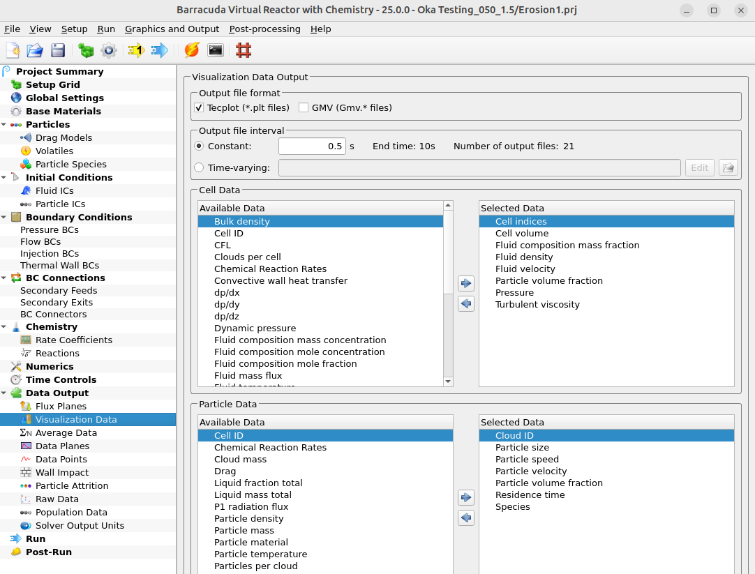
Figure 6: Data visualization window from Barracuda Virtual Reactor GUI
Run
- Click on Run and then click on Run Solver.
- Select GPU Parallel if you have the required GPU parallel license.
Post Processing Erosion Results in Tecplot
The user is assumed to have undergone basic Tecplot training, Getting Started With Tecplot For Barracuda® | CPFD Software (cpfd-software.com). So, only a few brief steps for post-processing the results are explained.
- In the Barracuda GUI, click on post-run and then click on View Results.
- Deselect Scatter from the Plot menu.
- The default units for erosion rate in Barraucuda are kg/m2/year. These units need to be converted into units for the penetration rate, which are m/kg. This can be done using the Specify Equations option in Tecplot.
- Got to Data. Select Alter and then Specify Equations.
- In the Specify Equations Box, select Wall Impact 002 from Data Set Info.
- Note that Tecplot requires all variable names to be enclosed in curly brackets in the Specify Equations editor. This includes Barracuda output variable names as well as user-defined variable names. Refer to the Tecplot help for more information on using the Specify Equations editor in Tecplot.
- The default Barracuda units for {Wall Impact 002} are kg/m2/year. This will first be converted into units of kg/m2/sec.
- To do this, define a new variable as {Wall_Impact_persec (kg/m2/sec)} = {Wall impact 002}/(365*24*60*60).
- Note that the kg in the units for Wall_Impact_persec (kg/m2/sec) refers to kilograms of sand particles impacting the surface. On the other hand, the kg in units for the penetration rate (m/kg) refers to kilograms of Aluminium solid wall material.
- The below steps outline the calculation of {Penetration_ratio} in units of m/kg from {Wall_Impact_persec} in units of kg/m2/sec.
- Divide {Wall_Impact_persec (kg/m2/sec)} by the mass flow rate of sand and the density of the solid wall material.
- {Penetration_ratio (m/kg)} = {Wall_Impact_persec (kg/m2/sec)} / (2.752e-4 * 2700). Where 2.752e-4 kg/sec is the mass flow rate of sand particles and 2700 kg/m3 is the density of the Aluminium solid wall material.
- While the density of Aluminium is available from the material properties definition, the mass flow rate of sand particles needs to be calculated. In the current setup, the air flow velocity and sand particle volume fraction are specified in the Velocity_inlet.sff. These values, along with the pipe inlet area (pipe diameter = 0.0254 m) and the specified slip ratio of 1, can be used to obtain the particle feed mass rate using the equation specified in section 8.1.3 (under Volume fraction heading) in the Barracuda help guide. This equation is shown below:
- In the Specify Equations Box, select Wall Impact 002 from Data Set Info.
$$\dot {m_p} = \dot{V_f} \cdot S \cdot \rho_{p} \frac{\theta_{p}} {1 – \theta_{p}} $$,
where \(\dot{m_p}\) = mass flow rate of sand particles, \(\dot{V_f}\) = volumetric flow rate of air, \(S\) = slip ratio, \(\rho_{p}\) = density of sand and \(\theta_{p}\) = volume fraction of sand particles
- Check Contour Box
- Click on settings beside Contour to open up the Contour & Multi-Coloring Details window.
- From the drop-down list, select Penetration_ratio (m/kg).
- From the drop-down list under Color map options, select Modified Rainbow – Less Green.
- Click on Set Levels and set the Minimum level to 2e-06, Maximum level to 2e-05, and Number of levels to 10 for the mass loading of 0.013
- Under the Color map distribution method, change the method to Continuous.
- For contour values at end points, enter 2e-06 for Min and 2e-05 for Max.
- Click on the Close button to close the Contour & Multi-Coloring Details window.
- Uncheck Translucency from under the Show Effects in the plot section on the left.
- Go to Plot and click on 3D Orientation Axis. Check the show 3D orientation axis box as shown in Fig 7.
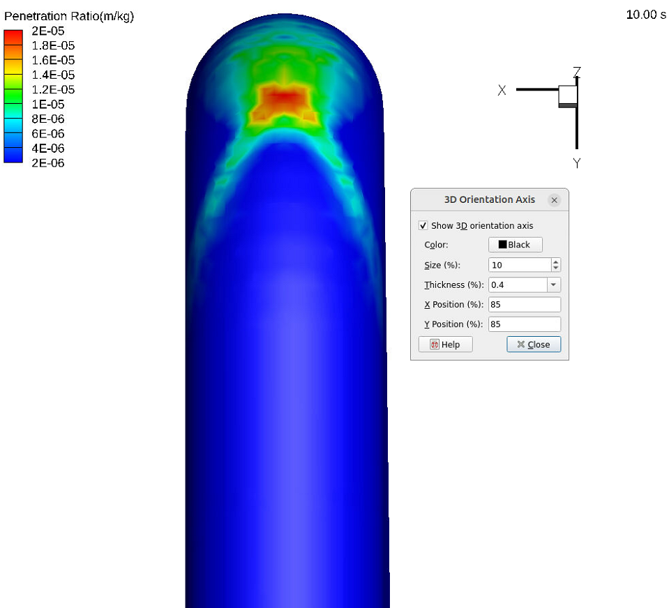
Figure 7: Default view of the Penetration Ratio contour plot.
6. Go to View and select Rotate. Enter 90 in the Rotation Step (degrees) dialog box and rotate the Z axis and X axis to get the view shown in Fig 8.
7. Go to Frame and click on Save Frame Style, and save the frame style with a desired name.
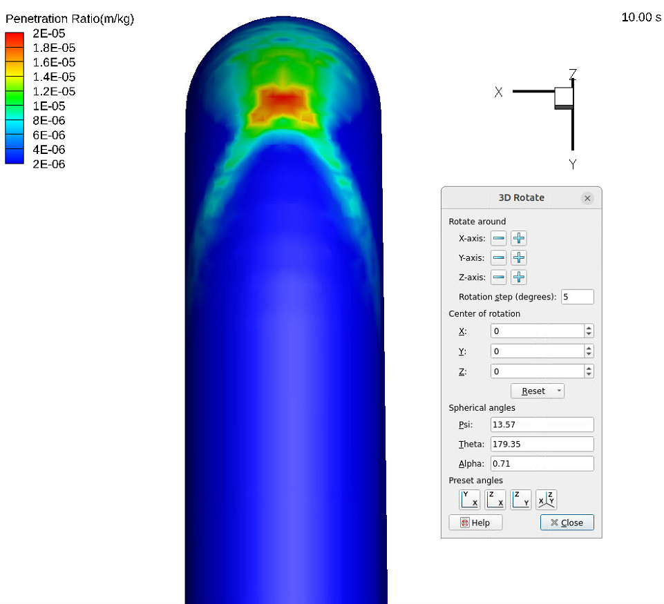
Figure 8: Adjusted view of the Penetration Ratio contour plot after step 6
Erosion Simulation Setup for Mass Loading of 1.5
The existing Erosion project file for a mass loading of 0.013 can be converted into a case with a mass loading of 1.5 as shown below.
- From the File menu, choose Save Case As. Save the project file as erosion_1p5_nocollision.prj in a different, newly created directory.
- Go to the Flow BCs window and click on edit transient file.
- Go to the Particle Volume Fraction tab and change the volume fraction from 6.12e-6 to 7.06e-4.
- Click on Run and then click on Run Solver.
As discussed above, for the case with mass loading of 1.5, particle collisions affect the erosion pattern (See Figure 4 discussion). To turn on the collision models in Barracuda, follow the steps below.
- From the File menu, choose Save Case As. Save the project file as erosion_1p5_collision.prj in a different, newly created directory.
- Go to View and check Beta Mode. Click on Particles in the selection tree.
- In the Particles window, check Enable equilibrium collision model, Enable isotropy collision model, as shown in Fig. 9.
- Click on Run and then click on Run Solver.
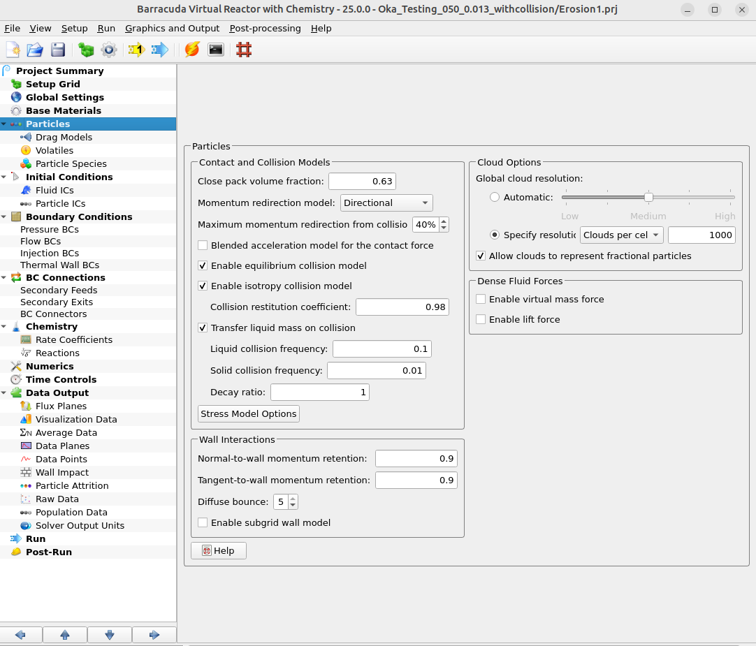
Figure 9: Collision models shown under Particles tab in the selection tree.
- The steps outlined in the Post Processing Erosion Results in Tecplot section can be used to post-process results for the mass loading = 1.5 case with and without particle collisions. Note that the mass flow rate of sand particles increases as the mass loading increases. This change in sand mass flow rate is listed below in the penetration ratio calculation.
- {Penetration_Ratio (m/kg)} = {Wall_Impact_persec (kg/m2/sec)} / (3.175e-2 * 2700). Where 3.175e-2 kg/sec is the mass flow rate of sand particles and 2700 kg/m3 is the density of the Aluminium solid wall material.
- Remember to save two separate Tecplot Frame Styles for cases without and with collision models turned on. These frames will be used in the next section to plot these results side-by-side in the same Tecplot window.
Plotting mass loading = 1.5, no collision results, to mass loading = 1.5, with collision results, together in Tecplot
To create the contour plot shown in Figure 4, follow the steps shown below.
- Tecplot frames can be used to show penetration ratio erosion contours for the mass loading = 1.5 case, with and without collisions, side-by-side. The user is expected to have already gone through the training material in “Tecplot for Barracuda – Using frames” (Tecplot for Barracuda – Using Frames | CPFD Software (cpfd-software.com)).
- Open a Tecplot session for the mass loading = 1.5 case without collisions
- Load the previously saved Frame style for this case. This should set up the view shown in Figure 8.
- From the top menu bar in Tecplot, select Frame ⇒ Create New Frame.
- Go to File and select Load Barracuda data, and then select Load 3D Data Set. Navigate to the working directory for mass loading 1.5, with collisions simulation, and select bvr.cells.0000.plt.
- Remember to load Tecplot files for all times by selecting All under Load Barracuda data ⇒ Tecplot Files to Load.
- Select Tile frames from Frame and tile the frames vertically.
- Select Frame ⇒ Frame Linking, and then check the boxes for Solution Time, 3D plot view.
- Load the previously saved frame style during the post-processing of the mass loading = 1.5 case with collisions
- Open a Tecplot session for the mass loading = 1.5 case without collisions
This concludes the description of the simulation setup process for Application Model: Erosion in a 90-degree elbow.
References
Oka, Y. I., Okamura, K., & Yoshida, T. (2005). Practical estimation of erosion damage caused by solid particle impact: Part 1: Effects of impact parameters on a predictive equation. Wear, 259(1-6), 95-101.
Oka, Y. I., & Yoshida, T. (2005). Practical estimation of erosion damage caused by solid particle impact: Part 2: Mechanical properties of materials directly associated with erosion damage. Wear, 259(1-6), 102-109.
Duarte, C. A. R., de Souza, F. J., & dos Santos, V. F. (2015). Numerical investigation of mass loading effects on elbow erosion. Powder Technology, 283, 593-606.
Mazumder, Q. H., Shirazi, S. A., & McLaury, B. (2008). Experimental investigation of the location of maximum erosive wear damage in elbows.