
Introduction
The evolution of cement manufacturing has transformed the industry from small-scale, energy-inefficient kilns to today’s advanced, automated preheater–precalciner systems, which maximize heat recovery, minimize fuel consumption, and increase the use of alternative fuels. This continuous technological progress has enhanced production efficiency, improved product quality, and improved environmental performance, laying the foundation for low-carbon and sustainable cement production in the modern era. Cement production, however, remains energy and carbon-intensive, contributing approximately 5% of global fossil CO₂ emissions from the calcination process alone (Andrew, 2019), and around 7–8% when fuel combustion is also considered (IPCC, 2014). This makes the cement sector a critical focus for innovation in efficiency, increased usage of alternative fuels, and lowering carbon emissions to meet global sustainability goals.
Figure 1 presents a schematic of the overall cement manufacturing process, encompassing raw material and coal preparation, pyroprocessing, preheater tower operation, gas cooling, dust filtration, and finished cement processing. Figure 2 focuses specifically on the pyroprocessing stage, in which raw materials are heated to high temperatures in the rotary kiln to form clinker, the principal component of cement; this stage involves the preheater tower, calciner, and rotary kiln.
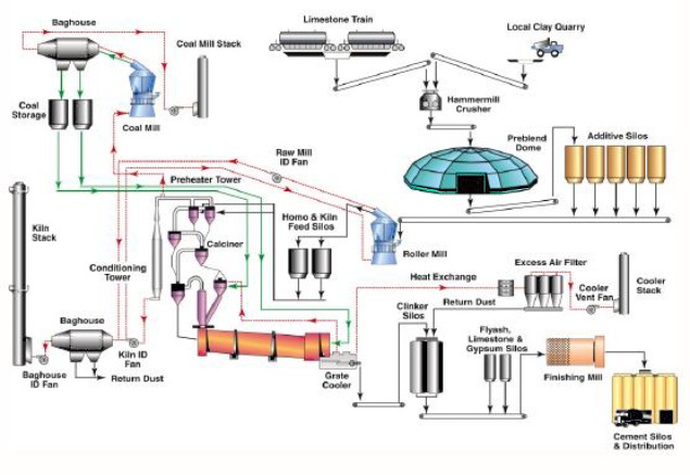 Figure 1: Typical Cement Manufacturing Process (Courtesy of Aixprocess, Barracuda Users Conference, 2019) |
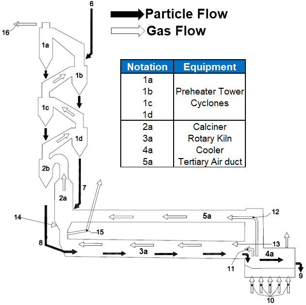 Figure 2: Cement Manufacturing Pyro-Processing Schematic |
The following process description primarily relates to the pyroprocessing process, as highlighted in Figure 2. Finely ground raw meal from the raw mills enters the four-stage preheater cyclones, where counter-current kiln/calciner exhaust gases heat it from ~50 °C to ~870 °C before it is dropped to the Calciner. The exhaust gases from the Calciner continue to the Conditioning Tower, where it is cooled and the entrained dust is filtered before being vented through the stack. Inside the Calciner, the fuel burns with Oxygen supplied by the Kiln exhaust gas and Tertiary air from the Cooler via the tertiary air duct, sustaining the high raw meal temperature and driving the Limestone (raw material) decomposition characterized by the main calcination reaction (CaCO₃ → CaO + CO₂). The exhaust gases with the entrained calcined material exit the calciner and enter the separation cyclone 2b. The calcined raw meal is separated from the gas in cyclone separator 2B via a vortex separation process. It is then discharged from the bottom and enters rotary kiln 3a through chute 8 for further processing before being converted into clinker.
Inside the slightly inclined kiln, the calcined raw meal is raised to ~1400 °C near the main burner (13). It undergoes clinkering reactions to produce cement clinker before being discharged to the grate cooler, where rapid air quenching lowers its temperature to ~150 °C. The heated cooler air serves as secondary air to the kiln burner and tertiary air to the calciner. A riser-duct bypass (15) can divert part of the Kiln exhaust gases when higher levels of circulating volatile gases are encountered in the kiln.
The cement calciner is the heart of the cement manufacturing process because it performs most of the raw material decomposition (CaCO₃ → CaO + CO₂); the process’s most energy-intensive step before the calcined raw meal is fed into the rotary kiln. By completing ~90–95% of calcination in the calciner, the rotary kiln is freed to focus on producing cement clinker, thereby increasing throughput, reducing specific fuel consumption, and stabilizing product quality. Moreover, the calciner can serve as a lever for the cement plant’s emissions and fuel flexibility. The inherently long residence times, coupled with turbulence-induced mixing, make the calciner an ideal place to co-process alternative fuels, such as Municipal Sludge, Biomass, Tire Chips, Natural Gas, and Refuse-derived fuels (RDFs). Due to the 90-95% calcination that occurs inside the Calciner and the resulting high CO₂ generation during the process, the Calciner is an ideal location for Carbon capture solutions.
The Barracuda Virtual Reactor (henceforth referred to as Barracuda) calciner model developed herein is primarily based on the work of Zhu et al. (2024), from which core model inputs and parameters are derived. Where specific inputs are unavailable in the primary source, assumptions are made based on prior process knowledge and open-source literature. In this post, we present the Barracuda model results for the calciner with coal and compare them with available cement plant data from Zhu et al. (2024).
The Barracuda Application model primarily simulates the hydrodynamics and relevant chemical reactions within the calciner, using coal as the primary fuel. The application model showcases the setup and CPFD (Computational Particle Fluid Dynamics) simulation of an industrial-scale cement calciner model with Barracuda, incorporating all relevant physics, and serves as a reference starting point for developing similar industrial-scale models with Barracuda. The model exemplifies the simulation of a compressible, thermally reacting, dynamic industrial system using Barracuda Virtual Reactor. Support files for the coal case are provided to registered users as an accompaniment to this post. These include the Barracuda Project file (containing the model setup and kinetics) and Post-processing templates for generating the qualitative results. Additionally, an Excel sheet is provided to assist users in estimating the volatile gas components released during devolatilization and determining the fuel composition.
To further extend the application of this work, a Barracuda model for simulating the co-processing of municipal waste sludge within a decomposition furnace has also been set up, incorporating the appropriate kinetics and model geometry, and is available for download as a reference. This model, with its parameters developed from the primary source (Zhu et al., 2024), offers a valuable starting point for exploring the sludge co-processing scenarios.
CPFD uses information from the literature for application model development, but does not independently verify its accuracy.
Model Description
The Barracuda calciner model incorporates a set of flow inputs and boundary conditions, primarily derived from Zhu et al. (2024), to simulate the cement calciner, also known as an industrial cement decomposition furnace. Gaseous species, such as the tertiary air and the kiln exhaust gas, enter the calciner through designated inlets. The raw material (pulverized limestone) and the coal fuel are modeled as a Solid species and enter the calciner through the designated inlets. The model domain begins downstream of the kiln exhaust and extends past the elbow to the calciner outlet. The calciner geometry for the Barracuda simulation is developed based on available literature and reasonable assumptions, as required. Figures 3 and 4 show the calciner geometry and the defined flow inlets and outlets, respectively.
The calciner features a narrow inlet for kiln exhaust gas that transitions conically into three stacked cylindrical sections designed to increase residence time, maximize gas-solid contact, and enhance heat transfer. Tertiary air is introduced eccentrically in the first cylindrical section, with coal pneumatically fed through four narrow 60° inclined pipes just below it. This staged introduction of fuel and hot air ensures efficient combustion, driving the main endothermic calcination reaction, which is the primary objective of the calciner. Preheated raw material (predominantly CaCO3) from the upstream preheater stage cyclone enters the calciner through a “splash-box” via multiple chutes along the cylindrical sections at two elevations, flowing counter-currently to the hot gas. Staging raw meal through two lower and two higher inlets distributes the endothermic load and solids holdup along the riser, improving gas–solid mixing and heat transfer. This results in smoother temperature and residence-time profiles, achieving the target calcination while minimizing temperature hotspots, material build-ups, and operability issues. The top culminates in an inverted tube structure serving as the calciner exit, facilitating gas-solid separation.
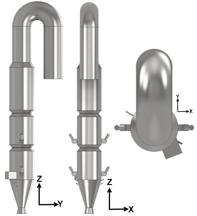
Figure 3: Barracuda Model of the Cement Calciner (Developed based on the work of Zhu et al. (2024))
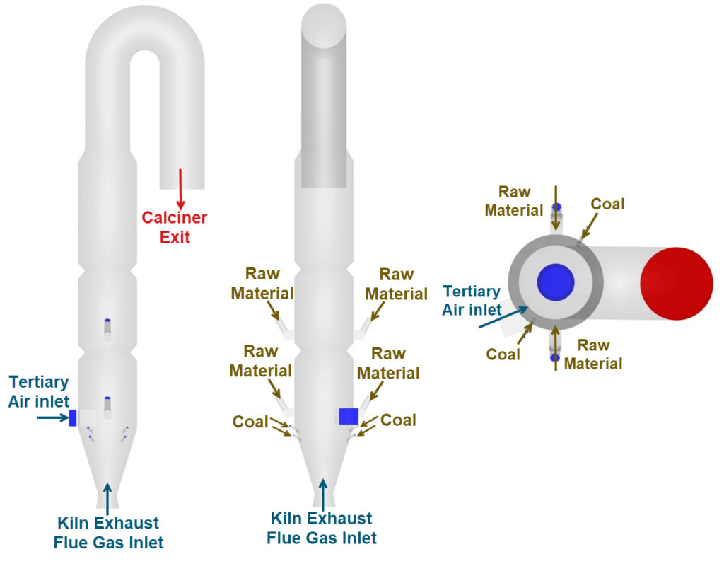
Figure 4: Barracuda Model Inlets and Outlet
Model Definition
The application model exemplifies the use of a compressible domain with reaction kinetics to model the devolatilization, oxidation, and calcination reactions inside the calciner. The flow boundaries (referred to as Flow BCs) are defined in Barracuda for gas and particle inlets, with specified inputs for mass flow rate, temperature, gas and particle compositions, and, if applicable, particle size distribution. A pressure boundary is defined at the outlet with a specified ambient pressure, allowing gas and solids to exit the domain without restriction, and is primarily driven by hydrodynamic forces. Thermal walls are defined to capture heat loss through the calciner’s outer walls by specifying an emissivity and a thermal wall resistance that depend on the wall material properties, thickness, and the presence of refractory, if any.
The raw material (mainly CaCO3 and CaO) and coal fuel are modeled as Solid species with appropriate PSDs and compositions. The materials are drawn from Barracuda’s built-in library, and the specified material properties, such as viscosity, heat capacity, and thermal conductivity, are temperature-dependent. The composition of coal, as estimated from proximate and ultimate analyses, is included in the Volatile Estimation Excel sheet provided in the support files. The calciner is initialized with 100% N2 at the expected outlet temperature of 1140 K and the outlet pressure of 99.83 kPa. Heat transfer through Convection, particle-to-particle conduction, and radiation is accounted for using the built-in models in Barracuda. Figure 5 illustrates the inputs used to define the flow boundary conditions (Flow BCs) for the solid and fluid boundaries.
The Beetstra drag model is used to capture the fluid-solid drag interaction for both the solid species.
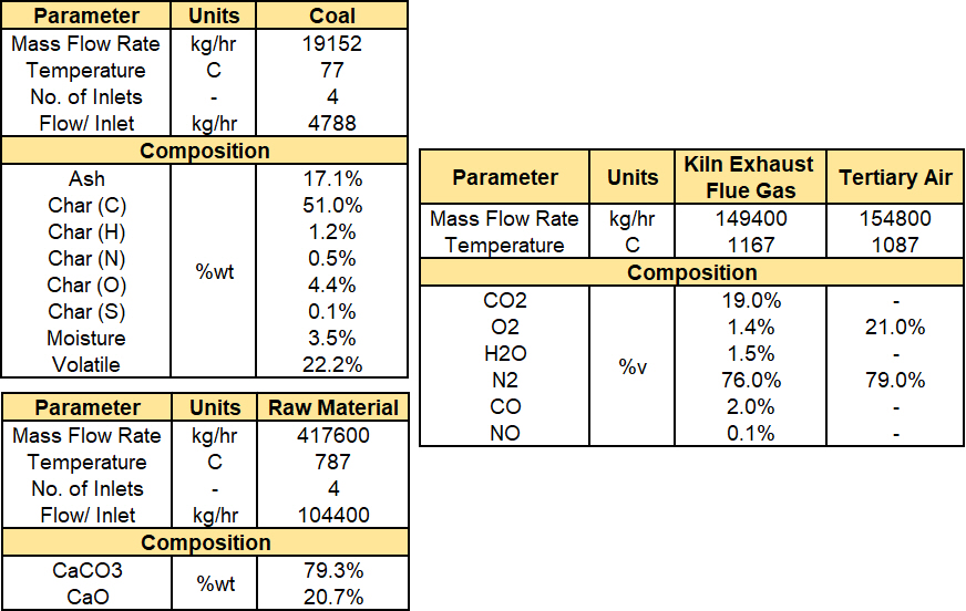
Figure 5: Barracuda Model Flow Inputs
Reaction Kinetics
The reaction kinetics implemented in the cement calciner incorporate Volume-averaged chemistry (represented as Stoichiometric reactions) to describe homogeneous gas-phase reactions, such as Methane oxidation, and heterogeneous gas-particle-phase reactions. A discrete-chemistry approach is used for particle-gas and particle-particle reactions, such as Calcination, Coke Oxidation, and Devolatilization. The reaction rate depends on temperature, pressure, fluid density, fluid volume fraction, and particle characteristics, such as size and composition. It can be described using Arrhenius reaction rate coefficients, polynomials, or user-defined expressions.
The reaction kinetics in this model are adopted from Zhu et al. (2024) and supplemented with data from open-source literature (Maya et al. (2018), Westbrook et al. (1981), Krusch et al. (2019), Molintas et al. (2022), Pang et al. (2021), Hashimoto et. al (2017), Zeng et al. (2021), de Bruyn Kops et. al (2004) ), for other physically significant reactions (e.g., methane combustion, H₂ combustion, CO oxidation). The combined kinetic scheme was then modified as needed to be compatible with Barracuda Virtual Reactor.
Figure 6 provides a snapshot of the reactions implemented in the Barracuda Application Model.
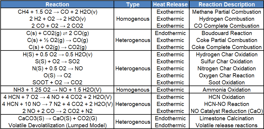
Figure 6: Chemical Kinetics Implemented in Barracuda
The devolatilization of the volatile component in the fuel is modeled with a lumped model approach. A “volatile” solid species is created with a Heat of Formation that is calculated as the net difference between the Heat of Formation of Devolatized products and Heat of Devolatilization, both estimated in the Volatile_Estimation_Template sheet. This sheet estimates the detailed distribution of volatile gases and char from coal using proximate and ultimate analysis data, ensuring full elemental and energy balance. It computes the devolatilized gas composition, char species, heat of devolatilization, and heats of formation of the reactants based on user-assumed splits of elemental nitrogen, hydrogen, and oxygen between volatile gases and char. Assumptions will need to be changed based on the system and the fuel accordingly. Instructions for estimating the volatile gas components and the composition of individual char species are provided in the Excel sheet.
A discrete reaction is set up to model this devolatilization by consuming a pseudo-solid species defined as “Volatile” at a rate proportional to its disappearance, and generating volatile gaseous products (CH₄, CO, CO₂, NH₃, HCN, H₂, H₂S, and Soot) at fixed mass fractions estimated in the volatile estimation sheet. The estimated “Volatile” heat of formation ensures that both mass and energy balances are accurately represented during particle devolatilization in the simulation.
The complete reaction set is provided in the support files and can be imported from the Barracuda Project file. These reactions can be a valuable starting point for modeling similar industrial systems, such as CFB boilers, Calciners, Gasifiers, and Chlorinators, with appropriate adjustments to the fuel composition, volatile gas composition, and reaction rate parameters.
The first set of reactions (1–7) in the kinetic model primarily occur in the gas phase and represent the oxidation and reduction processes of volatile species released during devolatilization, as well as the interactions between these volatiles and the flue gases exiting the kiln. Reactions (4), (5), and (6) describe the fuel-NOₓ formation and reduction pathways arising from the fuel-bound nitrogen. The oxidation of HCN leads to NO formation, while subsequent reactions among HCN, NO, and CO promote the reduction of NO to N₂, and CaO exhibits a strong catalytic effect on this reaction.
$$ CH_4 + 1.5 O_2 \rightarrow CO + 2 H_2O \quad \text{(1)} $$
$$ 2H_2 + O_2 \rightarrow 2 H_2O \quad \text{(2)} $$
$$ CO + 0.5 O_2 \rightarrow CO_2 \quad \text{(3)} $$
$$ 2NH_3 + 1.25 O_2 \rightarrow NO + 1.5 H_2O \quad \text{(4)} $$
$$ 4HCN + 7 O_2 \rightarrow 4 NO + 4 CO_2 + 2 H_2O \quad \text{(5)} $$
$$ 4HCN + 10 NO \rightarrow 7 N_2 + 4 CO_2 + 2 H_2O \quad \text{(6)} $$
$$ 2NO + 2 CO \rightarrow 3 CO_2 + N_2 \quad \text{(7)} $$
Reactions (8)–(11) represent the solid–gas phase reactions, encompassing the oxidation of char-bound species such as hydrogen, nitrogen, and carbon, as well as the release of bound oxygen from the solid matrix. These reactions collectively describe the conversion of solid-phase components into gaseous products during the oxidation of char.
$$ SOOT(s)+ O_2 \rightarrow CO_2 \quad \text{(8)} $$
$$ H(s) + 0.25 O_2 \rightarrow 0.5 H_2O \quad \text{(9)} $$
$$ N(s) + 0.5 O_2 \rightarrow NO \quad \text{(10)} $$
$$ O(s) \rightarrow 0.5 O_2 \quad \text{(11)} $$
$$ S(s) + O_2 \rightarrow SO_2 \quad \text{(12)} $$
Discrete reactions are defined to account for the devolatilization of Coal, Oxidation of Coke, and the Calcination of raw material (Limestone). The rate coefficients that capture reaction rate dependencies, such as pressure and temperature, are included as User-defined expressions in Barracuda and discussed in detail in the model setup section of this post. Reaction (13) describes the main endothermic calcination reaction. Reaction (14) and (15) describe the oxidation of coke to CO and CO2, with a split factor (φ) that controls the fraction of carbon oxidized to CO versus CO2. A smaller φ favors CO2, while a larger φ favors partial oxidation to CO. Reaction (16) describes the devolatilization of coal using a pseudo “Volatile” species written in the stoichiometric form purely for illustration. This reaction is implemented in the “species” form and described in the Chemistry section later in this post.
$$ CaCO_3 \rightarrow CaO + CO_2 \quad \text{(13)} $$
$$ C(s) + 0.5 O_2 \rightarrow CO \quad \text{(14)} $$
$$ C(s) + O_2 \rightarrow CO_2 \quad \text{(15)} $$
$$
\begin{aligned}
\text{Volatile(S)} \rightarrow &\; 0.372\,\text{CH}_4 + 0.375\,\text{CO} + 0.003\,\text{NH}_3 + 0.003\,\text{HCN} \\
& + 0.045\,\text{SOOT} + 0.045\,\text{H}_2 + 0.003\,\text{H}_2\text{S} \\
& + 0.185\,\text{CO}_2 \quad \text{(16)}
\end{aligned}
$$
The reaction rates for the above volume-averaged reactions (1-12) are shown below. The reaction rates for the discrete reactions (13-16) are omitted here and instead shown in the later sections of this post.
$$ R_1 = k_1 [CH_4]^{-0.3} [O_2]^{1.3} \quad \text{(1)} $$
$$ R_2 = k_2 [H_2]^{0.5} [O_2] \quad \text{(2)} $$
$$ R_3 = k_3 [CO] [H_2O(v)]^{0.5} [O_2]^{0.25} \quad \text{(3)} $$
$$ R_4 = k_4 [NH_3] [O_2] \quad \text{(4)} $$
$$ R_5 = k_5 [HCN] \quad \text{(5)} $$
$$ R_6 = k_6 [HCN] [NO] \quad \text{(6)}$$
$$ R_7 = k_7 [CO] [NO] \quad \text{(7)} $$
$$ R_8 = k_8 [SOOT] [O_2]^{0.5} \quad \text{(8)} $$
$$ R_9 = k_9 [O_2] \quad \text{(9)} $$
$$ R_{10} = k_{10} [O_2] \quad \text{(10)} $$
$$ R_{11} = k_{11} [O_2] \quad \text{(11)} $$
$$ R_{12} = k_{12} [O_2] \quad \text{(12)} $$
The rate coefficients below, which capture the key rate dependencies, can be in Arrhenius form or user-defined expressions, with units consistent with the source. The user-defined rate coefficients for the discrete reactions (13-16) are omitted from the list below and are provided in the model setup section later in the post.
$$ k_1 = 1.5 \times 10^{7} \exp\left(\frac{-15098}{T} \right) \tag{1} $$
$$ k_2 = 1.6 \times 10^{9} \exp\left(\frac{-10000}{T} \right) \tag{2} $$
$$ k_3 = 3.98 \times 10^{14} \exp\left(\frac{-20130}{T} \right) \tag{3} $$
$$ k_4 = 3.1 \times 10^{08} \exp\left(\frac{-10000}{T} \right) \tag{4} $$
$$
\begin{aligned}
k_5 &= 1.0\times10^{11}\,\rho_{g}\,Y_{O_2}^{\,b}\,
\exp\!\left(-\frac{33700}{T_g}\right)\,\frac{1}{MW_{NO}} \quad \text{(5)} \\
\text{where: } & b\ \text{is the oxygen reaction level;} \\
& \rho_{g}\ \text{is the gas mixture density;} \\
& Y_{O_2}\ \text{is the mass fraction of oxygen;} \\
& T_{g}\ \text{is the temperature of the gas mixture;} \\
& MW_{NO}\ \text{is the molecular weight of NO.}
\end{aligned}
$$
$$
\begin{aligned}
k_6 &= 3.0\times10^{12}\,\rho_{g}\,\exp\!\left(-\frac{30000}{T_g}\right)\,\frac{1}{MW_{NO}} \quad \text{(6)} \\
\text{where: } & \rho_{g}\ \text{is the gas mixture density;} \\
& T_{g}\ \text{is the temperature of the gas mixture;} \\
& MW_{NO}\ \text{is the molecular weight of NO.}
\end{aligned}
$$
$$
\begin{aligned}
k_7 &= 3.9816\times10^{9}\,\rho_{g}\,\exp\!\left(-\frac{8920}{T_g}\right)\,Y_{CaO}\,\frac{1}{MW_{NO}} \quad \text{(7)} \\
\text{where: } & \rho_{g}\ \text{is the gas mixture density;} \\
& T_{g}\ \text{is the temperature of the gas mixture;} \\
& Y_{CaO}\ \text{is the mass fraction of CaO;} \\
& MW_{NO}\ \text{is the molecular weight of NO.}
\end{aligned}
$$
$$
k_8 = 3.9 \times 10^{6}\,\exp\!\left(-\frac{16959}{T_g}\right) \quad \text{(8)}
$$
$$
\begin{aligned}
k_9 &= 1.03 \times 10^{5}\,\exp\!\left(-\frac{18000}{T_g}\right)\,a_{h} \quad \text{(9)} \\
\text{where: } & a_{h}\ \text{is the area of Hydrogen in the char.}
\end{aligned}
$$
$$
\begin{aligned}
k_{10} &= 7.36 \times 10^{2}\,\exp\!\left(-\frac{18000}{T_g}\right)\,a_{n} \quad \text{(10)} \\
\text{where: } & a_{n}\ \text{is the area of Nitrogen in the char.}
\end{aligned}
$$
$$
\begin{aligned}
k_{11} &= 6.44 \times 10^{2}\,\exp\!\left(-\frac{18000}{T_g}\right)\,a_{o} \quad \text{(11)} \\
\text{where: } & a_{o}\ \text{is the area of Oxygen in the char.}
\end{aligned}
$$
$$
\begin{aligned}
k_{12} &= 3.22 \times 10^{2}\,\exp\!\left(-\frac{18000}{T_g}\right)\,a_{s} \quad \text{(12)} \\
\text{where: } & a_{s}\ \text{is the area of Sulfur in the char.}
\end{aligned}
$$
Results and Discussion
The results from the Barracuda calciner model for the coal case are compared with the available field data provided in Zhu et al. (2024). The calcination percentage (a measure of the decomposition of CaCO3 to CaO) and the gas temperature at the Calciner outlet, as available from field data measurements, are used for comparison with Barracuda results.
Figure 7 presents a comparison of these quantities as histograms. The Barracuda predictions show agreement with the plant data for both the outlet gas temperature and the degree of raw-meal calcination. This agreement indicates that the model reasonably reproduces the coupled gas–solid heat transfer and the kinetics of raw material (primarily CaCO₃) decomposition under industrial operating conditions. Furthermore, the implemented devolatilization, combustion, and calcination kinetics are adequate in capturing the heat-transfer characteristics and the overall energy balance of the calciner, as evidenced by the comparison with plant data. The reaction kinetic set implemented in the Calciner can therefore be reused if desired to model similar systems, with appropriate adjustments made to the kinetic parameters, such as rate constants, activation energies, and pre-exponential factors, to reflect material- and process-specific conditions.
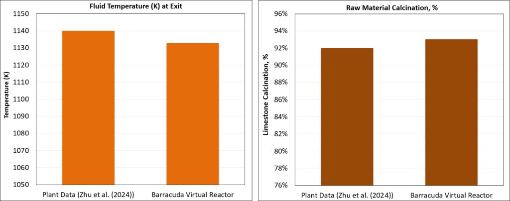
Figure 7: Comparison of Barracuda Results with Plant Data (Zhu et al., 2024)
Figure 8a illustrates the calcination of the raw material (CaCO₃ → CaO) in the calciner as predicted by the Barracuda model. The animation represents the fraction of total calcium present as CaO relative to the combined calcium content (CaO + CaCO₃). The raw meal entering the calciner through four feed chutes at two elevations is partially precalcined, and approximately 32 % of the total calcium is already present as CaO, due to heat transfer occurring in the upstream preheater stages. Calcination is a highly endothermic process that begins at temperatures above 850 °C. As the raw material is entrained into the high-temperature zone of the calciner, it is heated by the energy released from exothermic coal combustion and undergoes progressive decomposition to CaO. The transient gas–solid flow and complex hydrodynamics within the furnace influence the local temperature field and residence time, resulting in spatial variations in the degree of calcination both axially and radially. The animation indicates a gradual axial increase in calcination as the raw material is heated and undergoing decomposition, with conversion peaking in the third cylindrical chamber and the inverted U–bend section, where the overall degree of calcination reached ~93% at the outlet.
The animation shown in Figure 8b illustrates the strong coupling between the raw material temperature, degree of calcination, and heat transfer. As the raw material gets heated up by the combustion of coal, the calcination of uncalcined raw material begins and accelerates as the temperature continues to increase along the reactor height.
A poorly designed calciner with inefficient heat transfer will result in a higher degree of uncalcined raw material leaving the system, which has a detrimental impact on downstream processes, such as clinker formation in the kiln, and cumulatively represents poor heat recovery in cement manufacturing.
The instantaneous spatial distribution of Oxygen in the Calciner over time is shown in Figure 9. The axial distribution is visualized by 2D planes created along X and Y directions, while the radial distribution is visualized with equally spaced planes along the reactor elevation. The O2 for combustion and oxidation reactions is primarily supplied through the tertiary air duct. As the tertiary air enters the calciner, oxygen (O2) is rapidly depleted by the combustion and oxidation reactions. The coal injected slightly below the tertiary air duct is carried upwards by the hot kiln exhaust gas and meets the O2-rich tertiary air, resulting in violent combustion reactions that cause peak temperatures to occur in the lower cylindrical sections. This provides the necessary energy for the main endothermic calcination reaction of limestone decomposition.
Figure 10 presents the predicted instantaneous CO₂ mole-fraction distribution inside the calciner. Elevated CO₂ concentrations are observed along the main calcination and combustion zones, where both the coal combustion and the decomposition of CaCO₃ contribute to CO₂ generation. The spatial gradients in CO₂ concentration correlate with the regions of high temperature, O₂ depletion (due to CO and Coke oxidation to CO₂), and active gas–solid interaction, indicating efficient coupling between combustion and calcination reactions. The introduction of Tertiary air (characterized by the absence of CO2) aids the combustion reaction and promotes localized dilution of CO2 through improved mixing and secondary oxidation of CO to CO2.
As the raw meal continues to decompose while ascending through the furnace, the CO₂ mole fraction progressively increases along the reactor height, reaching its highest values near the outlet. This trend aligns well with the predicted calcination degree exceeding 90% at the outlet, further confirming that the model captures the strong coupling and the overall mass and energy balance within the industrial calciner.
Figure 11 shows the instantaneous axial and radial temperature distribution over time within the calciner. A progressive decrease in gas temperature is observed with increasing elevation beyond the high-temperature combustion zones, primarily due to heat transfer from the hot flue gases to the colder incoming raw material. The raw meal enters at a relatively low temperature and absorbs heat from the exothermic combustion of coal volatiles and char, as well as from the surrounding gas phase. At higher elevations, the temperature distribution becomes more uniform, indicating that a local thermal equilibrium is established between the gas and solids. In this region, the calcination reaction rate and the endothermic heat demand of CaCO₃ decomposition are balanced by the available heat from combustion and particle–gas heat exchange, resulting in a nearly steady temperature band that persists toward the outlet.
Figure 12 illustrates the time-averaged NOx distribution in the calciner. At temperatures of 800 °C to 1200 °C inside the calciner, thermal and prompt NOx generation is negligible compared to the fuel NOx, which originates from the oxidation of nitrogen compounds present in the fuel (coal, sludge, and volatiles such as HCN and NH₃) and kiln exhaust gas. Fuel-NOₓ formation dominates in the lower combustion region where oxygen availability is high and temperatures range between 1000–1300 °C. At higher elevations, with reduced oxygen and higher levels of CO2, the reduction of NO to N2 is favored through reactions 6 (HCN + NO > N2) and 7 (NO + CO > N2), with the elevated levels of CaO in this region serving as a catalyst.
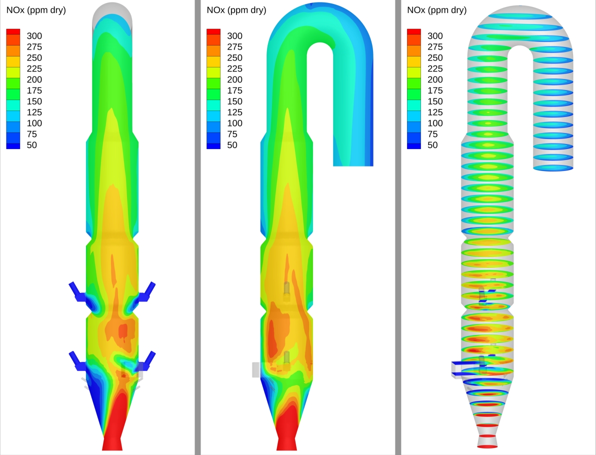
Figure 12: NOx distribution in the calciner predicted by Barracuda
Modeling Instructions
The user is expected to have already gone through basic Barracuda training: Barracuda Virtual Reactor New User Training | CPFD Software (cpfd-software.com).
- Download the support files provided along with this post.
- Unzip the support file and place it in the new folder created for running this Cement Calciner application model.
- Open a new Barracuda session.
- From the File menu, choose Open Project. Navigate to the working directory and select Cement_Calciner_BVR_AppModel.prj.
The project file has already been set up with the appropriate inputs and includes the following.
- Grid
- Base Materials.
- Particles.
- Initial Conditions
- Fluid ICs.
- Particle Species.
- Boundary Conditions
- Pressure BC at the Calciner outlet for gas and particle exit.
- Flow BCs for flow inlets.
- Thermal Wall BCs – Account for heat loss through the Calciner walls.
- Heat Transfer
- Particle-to-Particle Heat Conduction
- P-1 Radiation Model
- Chemistry Setup
- Post Processing
- Visualization Data
- Average Data
- Flux Plane
The reaction kinetics for this project, which are already set up under the Chemistry section in the project file, are described below.
Chemistry
To model the various reactions occurring in the cement calciner, a total of 15 reactions involving only gas, gas-particle, and particle-particle phases are considered. Several of the rate coefficients in the kinetic model (such as k1) follow the standard Arrhenius form, only requiring a pre-exponential factor (Co or A) and an activation energy (\( E = E_a / R \)) to be specified. These can be defined using the Chemistry Coefficient Editor with the Arrhenius Chem Rate built-in editor, which includes options for incorporating the dependence of fluid-only parameters, such as temperature, pressure, density, and volume fraction, as well as particle parameters, including volume fraction, mass, and area. The User-defined expression feature can also be used to define the rate coefficient in the Arrhenius form or any other form (such as polynomial or table-based chemistry), while maintaining consistency with the expected units of the reaction rate. Both approaches are adopted in this application model. For reactions with reaction rates dependent on fluid and particle parameters that have complicated dependencies, the user-defined expression feature in Barracuda is recommended for defining the rate coefficient.
The built-in evaporation model is enabled to account for the evaporation of moisture in the fuel. The default values are left unchanged in the model.
Volume-averaged reactions (1-4, 8-12) employ a simple Arrhenius-type rate coefficient, which involves specifying a pre-exponential factor, activation energy, and dependence on individual particle area for some. The instructions below describe the setup of the rate coefficient, $k_{12}$, for reaction (12), which is used as an example.
- Under Chemistry, select Rate Coefficients. Click Add to bring up the Chemistry Coefficient Editor. Volume-Average, which is the default reaction type, is used for this rate constant.
- Add the following equation parameters shown in Figure 7.
- Enter a value of \( 3.22 \times 10^{2} \) for \( C_0 \), the pre-exponential factor.
- Specify an activation energy of 18,000. Please note this value corresponds to \( E = E_a / R \).
- Select Particle Dependence in the Chemistry Coefficient Editor
- From the Project Materials List, add ‘S’ to the Materials List, selecting “area” for the Material Coefficient Type, and keep the exponent on the material as 1.
- Select an area unit of m2/m3.
Some volume-average reactions (5-7) involve a more complicated dependence of fluid and particle parameters on the rate coefficients. The User-defined Expression feature is most convenient for such reactions, and Figure 13 illustrates the expression for defining the rate coefficient of reaction (5), which involves the oxidation of the volatile fuel component HCN. The complexity involved in defining the dependence of oxygen reaction level on oxygen concentration, based on specific conditions, makes this a convenient approach.
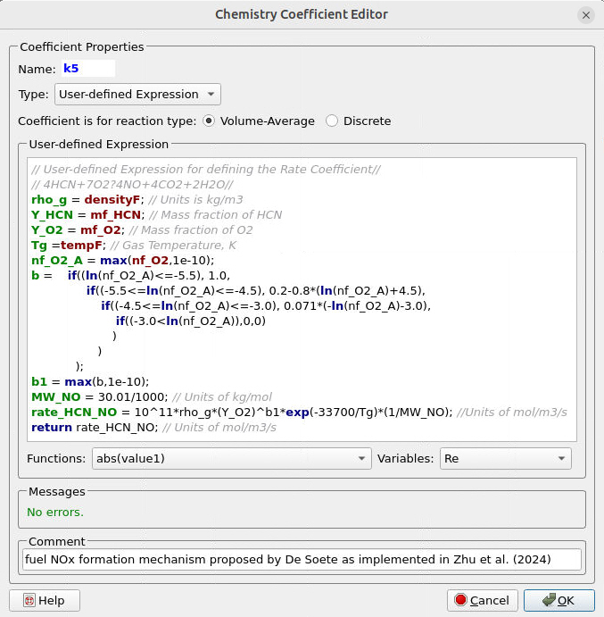
Figure 13: User-defined Rate coefficient in Barracuda
Discrete reactions (13-16) use a user-defined rate coefficient to capture rate dependencies. These reactions correspond to limestone calcination, coke oxidation, and devolatilization. Figure 14 illustrates the reaction rate and the corresponding rate coefficient for the calcination of the raw material. As \( CaCO_3 \) decomposes, \( CO_2 \) gas and \( CaO \) solids are produced at the same rate. Calcination rate is controlled by the intrinsic Arrhenius kinetics at the particle temperature, and suppressed by the \( CO_2 \) partial pressure relative to the temperature-dependent equilibrium pressure. The net calcination rate is scaled by the amount of \( CaCO_3 \) present in the calciner.
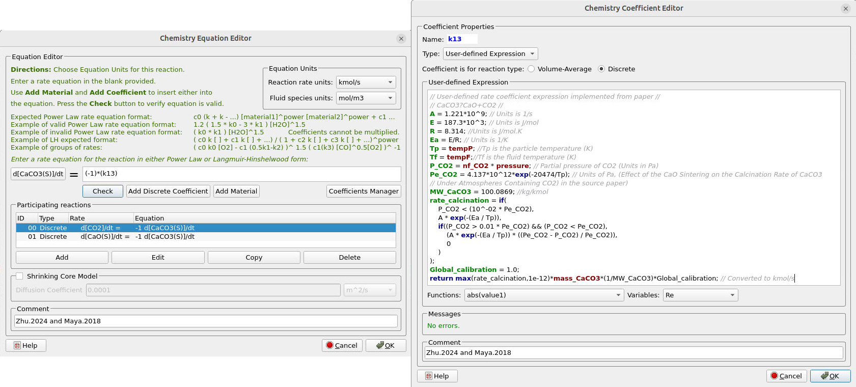
Figure 14: Reaction rate and rate coefficient for the calcination of raw material
Figures 15a and 15b illustrate the reaction rate and the rate coefficient for reactions (14) and (15), which correspond to the oxidation of Coke. The reaction employs a split factor, ɸ, which affects the conversion of Coke to \( CO \) and \( CO_2 \), respectively.
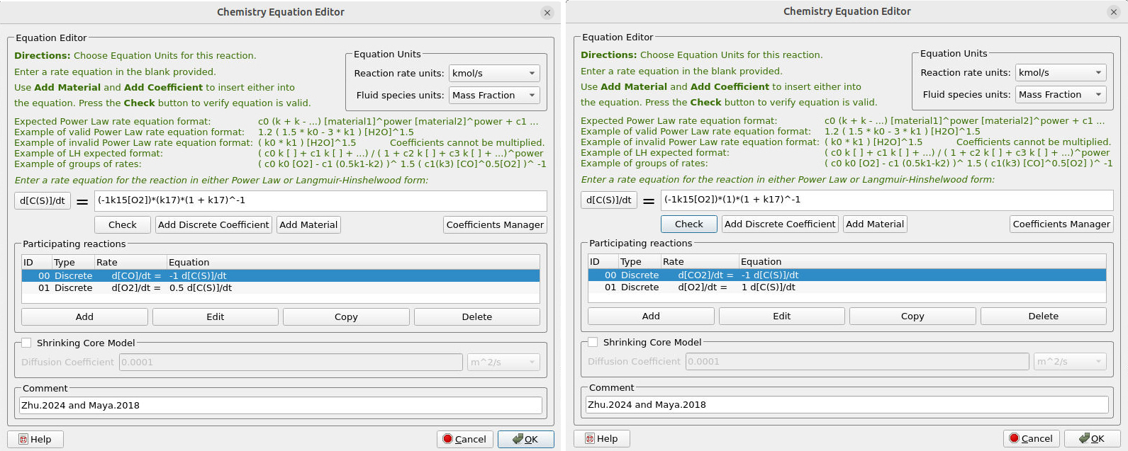
Figure 15a: Reaction Rate for Coke (C) Oxidation to CO and CO2
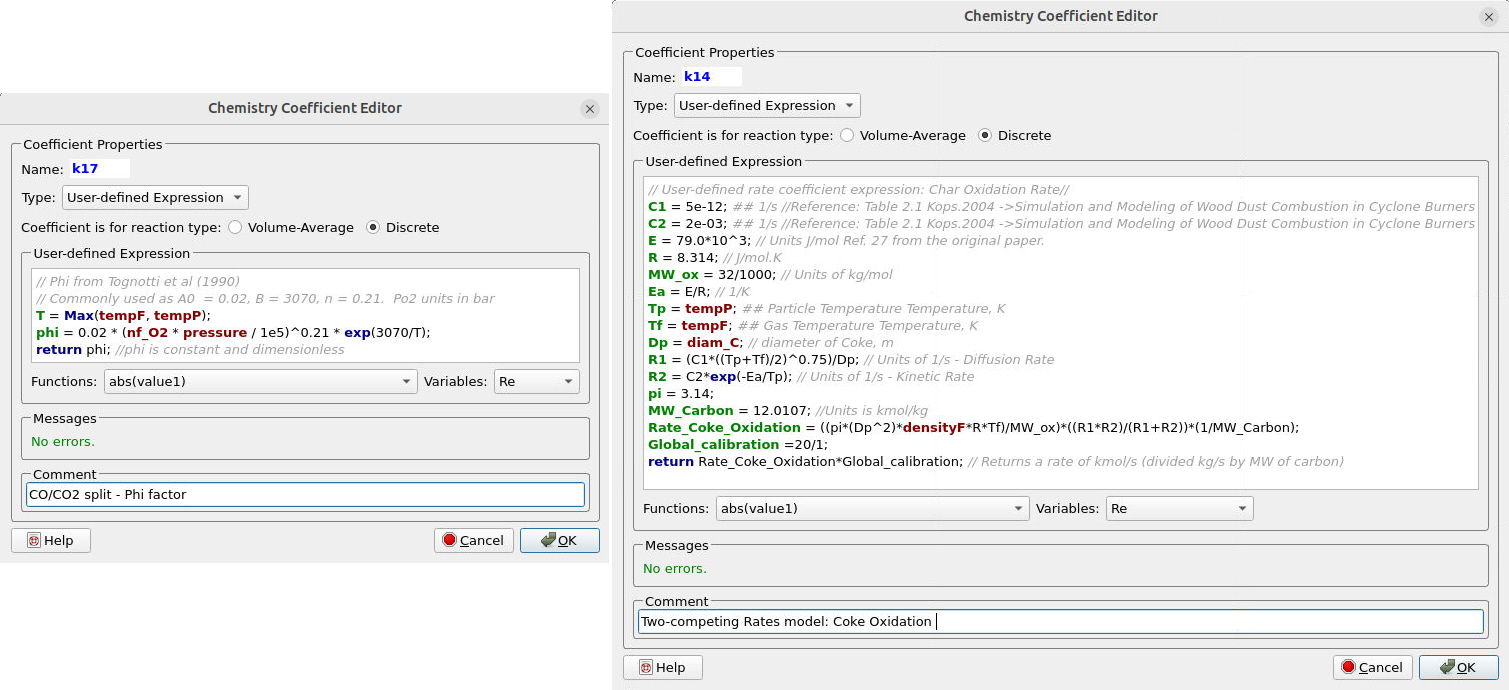
Figure 15b: Rate coefficient for the Coke Oxidation
Figure 16 illustrates the reaction rate and the corresponding rate coefficient for the devolatilization. As explained previously, a “pseudo” solid species, “Volatile,” releases the volatile gas components upon devolatilization. The composition of the volatile gases is estimated from the “Volatile_Estimation_Template” Excel sheet.
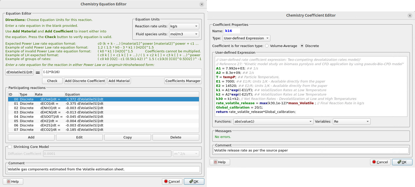
Figure 16: Reaction rate and rate coefficient for devolatilization of Coal
Time Controls
- Enter 0.01 seconds for the Time Step and 300 seconds for the End Time.
- Set the Restart Interval to 100 seconds.
Data Output
Verify that the checkboxes for the Mass.log and Energy.log outputs are enabled.
Data Points
Data points can serve as virtual probes to measure temperature, pressure, and other dependent variables. These are often used as a basis for comparison with experimental or plant data. Six data points are collected at the Calciner outlet to monitor fluid temperature and serve as a basis for comparison with the plant data provided in Zhu et al. (2024).
Visualization Data
Ensure that the following Visualization Data outputs are selected in the Visualization Data tab in Figure 10.
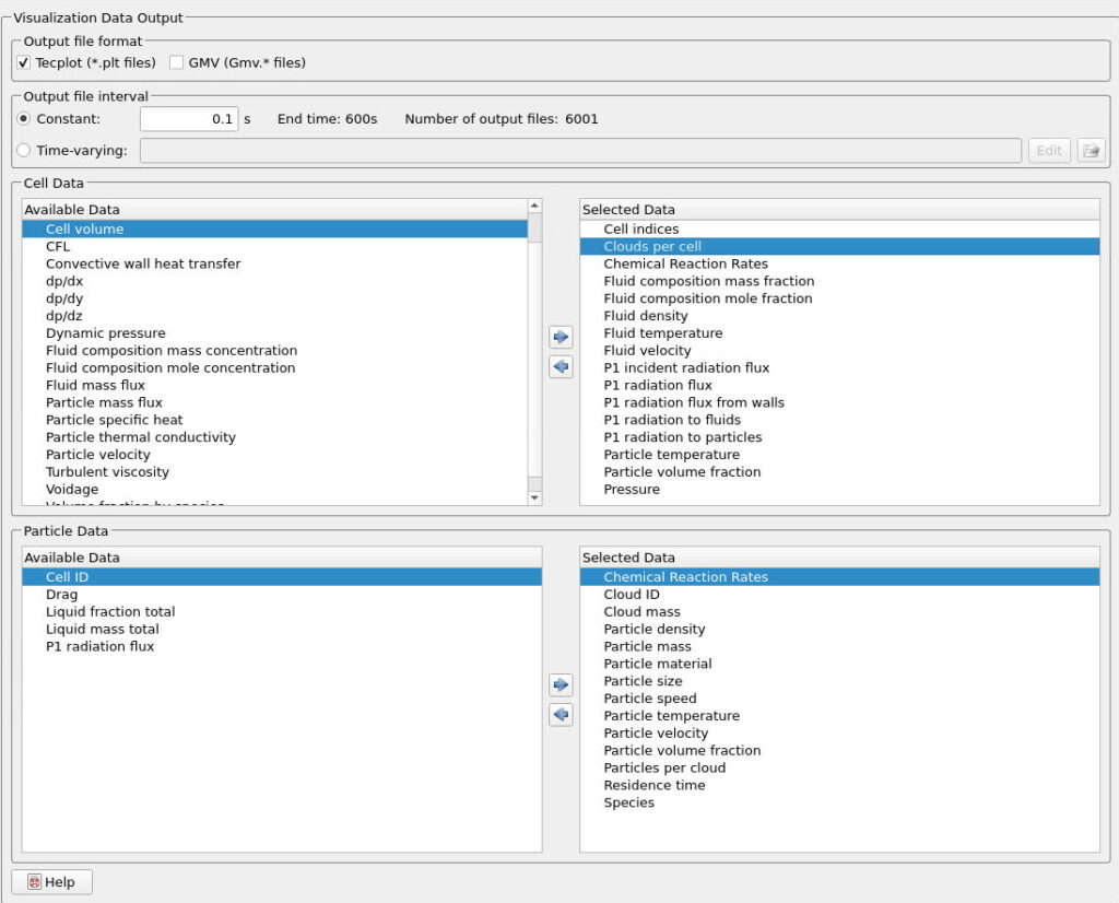
Figure 8: Visualization Data Output in Barracuda
Run
- Click on Run and then click on Run Solver.
- Select GPU Parallel if you have the required GPU parallel license.
Post-Processing Results
With Tecplot:
The user is assumed to have completed basic Tecplot training, Getting Started With Tecplot For Barracuda® | CPFD Software (cpfd-software.com), to familiarize themselves with basic operations in Tecplot. The gas and particle animations and snapshots shown in the results section can be generated easily using Tecplot style files (.sty). These templates are used to save and reuse the visual styling of a single plot frame, such as colors, line types, contours, and solid profiles. The templates are provided in the Downloads accompanying this post. The following steps are required to create a contour-style plot (e.g., Figure 9) and a solids profile (e.g., Figures 8a, and 8b) in Tecplot. The remaining visualizations follow similar instructions and are not further detailed.
To create the animation contour plot shown in Figure 9, follow the steps below.
- In the Barracuda GUI, click on Post-Run and then click on View Results.
- Deselect Scatter from the Plot menu.
- Select the checkbox next to Slices.
- Select the gear icon next to Slices.
- Under ‘Definition’, ensure that ‘X-planes’ is selected from the Drop-down menu.
- Under the Contour tab, select the key icon to open the Contour and Multi-coloring details window.
- Under the drop-down, select Fluid domain mole fraction O2(G)
- Under Color map options, select Modified Rainbow less green from the drop-down window.
- Select Continuous under the Color map distribution method. Note that the minimum and maximum values under ‘Contour values at endpoints’ will need to be manually updated based on the minimum and maximum values for the Contour legend. Set reasonable limits to visualize oxygen consumption.
- Under the plot sidebar, select the ZY view from the list to get the appropriate view.
- Select Frame -> Save frame style and save the frame style under a recognizable name, such as Oxygen_Contour_Slices_ZY.sty.
- Now that a single style file has been generated, the frame style can be used to create the equivalent view for other fluid species.
- Select the frame and press Ctrl + C to copy the frame. Create a copy of the same frame using Ctrl + V. The copying and pasting of the frames is repeated twice more, creating a total of 3 frames.
- Once all relevant frames have been generated, select Frame> Tile Frames and choose the side-by-side view from the dropdown list to tile and organize the frames.
- Next, double-click the contour bar on the second frame and select Fluid domain mole fraction O2(G) to view the results for the O2 mole fraction. Adjust min/max values in the Levels and Color tab as needed, ensuring that the bounds are also changed in the Color map distribution method window (below Color map). Under ‘Definition’, select ‘Y-Planes’ under the Drop-down menu.
- For the third frame, select the checkbox next to Slices.
- Select the gear icon next to Slices.
- Under ‘Definition’, ensure that ‘Z-planes’ is selected from the Drop-down menu.
- Select the checkbox labeled “Show start/end slices.”
- Set the Start slider to the minimum value and the End slider to the maximum value.
- Select Show intermediate slices, and enter the number of slices as 40 or another number as desired.
- Steps 1-10 can be used to create other key qualitative results, such as contours of Fluid Temperature, Velocity, and Gas compositions of CO, NOx, etc.
To create the view of the solids profiles, such as the one shown in Figures 8a and 8b, follow the steps shown below:
- In the Barracuda GUI, click on Post-Run and then click on View Results.
- Select Plot -> Blanking -> Value Blanking.
- Select the Include value blanking checkbox. We want to exclude all Solid species except the Raw Material to focus on visualizing the main endothermic Calcination Process inside the Calciner.
- Under Constraint 1, use the dropdown menu under Blank when to specify that Species should be blanked when it is greater than 4. Ensure that the Active checkbox is selected. This removes coal species from the visualization, showing only the raw material.
- Under Data-> Alter-> Specify Equations->Load Equations, load the AbsoluteCalcinerPerformance.eqn (provided in the support files) and click on Compute.
- Select the ZY view from the Plot sidebar to fit the Calciner in the frame.
- Double-click on the geometry to open the Zone Style window. Navigate to the Scatter tab.
- On the zone titled Particles, which should be Group 1, right-click on the highlighted Symbol shape. By default, it should be set to Point. From the list of options, select Sphere.
- Right-click on the Scatter size and select 0.75. This should significantly increase particle size and render them spherical.
- Double-click on the contour legend, and select Absolute_Calciner_Performance from the dropdown menu. Set the minimum and maximum values to 0 and 100, with a contour level delta of 5.
- Now that the spheres have been correctly generated, select Frame -> Save frame style and choose a name for the frame, such as AppModel_Calcination_View_ZX.sty. This can be used in the future to quickly generate the same frame view.
- Copy and paste the frame in the manner shown in the previous section.
- In the newly created frame, double-click the contour legend and select Absolute_Calciner_Performance from the dropdown list in the Contour and Multi-Coloring Details tab. This same view can be generated for all of the solid species.
- Select the ZX view from the Plot sidebar to fit the Calciner in the frame.
- Once all relevant frames have been generated, select Frame> Tile Frames and choose the “Side by Side” view from the dropdown list to tile and organize the frames.
- Steps 1-4 can be repeated, and for Step 5 under Data -> Alter -> Specify Equations -> Load Equations, load the RelativeCalcinerPerformance.eqn file, then click Compute.
- Steps 6-15 can be repeated to create the animation shown in Figure 8b.
Quantitative results, such as the raw material calcination % and the calciner outlet temperature, are estimated using Python scripts based on the FLUX plane data generated at the Calciner outlet pressure boundary. This concludes the application model for the calciner thermal-decomposition furnace.
References
IPCC, 2014: Climate Change 2014: Mitigation of Climate Change. Contribution of Working Group III to the Fifth Assessment Report of the Intergovernmental Panel on Climate Change [Edenhofer, O., R. Pichs-Madruga, Y. Sokona, E. Farahani, S. Kadner, K. Seyboth, A. Adler, I. Baum, S. Brunner, P. Eickemeier, B. Kriemann, J. Savolainen, S. Schlömer, C. von Stechow, T. Zwickel and J.C. Minx (eds.)]. Cambridge University Press, Cambridge, United Kingdom and New York, NY, USA
Zhu, L., Mao, Y., Liu, K., Tong, C., Liu, Q., & Xie, Q. (2024). The Co-Processing Combustion Characteristics of Municipal Sludge within an Industrial Cement Decomposition Furnace via Computational Fluid Dynamics. Mathematics, 12(1), 147.
Maya, J. C., Chejne, F., Gómez, C. A., & Bhatia, S. K. (2018). Effect of the CaO sintering on the calcination rate of CaCO3 under atmospheres containing CO2. AIChE Journal, 64(10), 3638-3648.
Westbrook, C. K., & Dryer, F. L. (1981). Simplified reaction mechanisms for the oxidation of hydrocarbon fuels in flames. Combustion science and technology, 27(1-2), 31-43.
de Bruyn Kops, S. M., & Malte, P. C. (2004). Simulation and Modeling of Wood Dust Combustion in Cyclone Burners. Energy and Environmental Combustion Laboratory.
Krusch, S. (2019). Experimental examination and simulation of a pilot-scale circulating fluidized bed reactor (Doctoral dissertation, Bochum, Ruhr-Universität Bochum, 2018).
Xie, J., Zhong, W., Jin, B., Shao, Y., & Liu, H. (2014). Three-dimensional Eulerian–Eulerian modeling of gaseous pollutant emissions from circulating fluidized-bed combustors. Energy & Fuels, 28(8), 5523-5533
Tighe, C. J., Twigg, M. V., Hayhurst, A. N., & Dennis, J. S. (2016). The kinetics of oxidation of Diesel soots and a carbon black (Printex U) by O2 with reference to changes in both size and internal structure of the spherules during burnout. Carbon, 107, 20-35.
Molintas, H. J., & Gupta, A. K. (2022). Combustion of Flat-Shaped Char Particles With Oxygen. Journal of Energy Resources Technology, 144(2), 022302.
Pang, L., Shao, Y., Zhong, W., & Liu, H. (2021). Experimental study and modeling of oxy-char combustion in a pressurized fluidized bed combustor. Chemical Engineering Journal, 418, 129356.
Hashimoto, N., Watanabe, H., Kurose, R., & Shirai, H. (2017). Effect of different fuel NO models on the prediction of NO formation/reduction characteristics in a pulverized coal combustion field. Energy, 118, 47-59.
Zheng, Y., Guo, Y., Wang, J., Luo, L., & Zhu, T. (2021). Ca doping effect on the competition of NH3–SCR and NH3 oxidation reactions over vanadium-based catalysts. The Journal of Physical Chemistry C, 125(11), 6128-6136.