
Introduction
Molten metal bubble column reactors (MMBCRs) have emerged as a promising technology for various chemical processes, particularly in the field of hydrogen production and carbon capture. These reactors offer several advantages over traditional methods, making them a subject of extensive research and development. Production of hydrogen using MMBCRs through non-oxidative CH4 (methane) pyrolysis is appealing because it’s inherently a low-carbon-emission technology. Thermal cracking of CH4 produces solid carbon and H2 without CO2. However, commercializing MMBCRs for CH4 pyrolysis has challenges associated with (i) developing materials that can withstand high temperatures and pressure and corrosive nature of molten metals; (ii) understanding and optimizing bubble dynamics, which influence reactor efficiency; and finally (iii) the effects of temperature, gas flow rates, and reactor geometry on conversion efficiency. Researchers have observed that in MMBCRs, decomposition of CH4 happens inside bubbles and on bubble (liquid-gas) interfaces, such that each bubble can be thought to act as an individual microreactor. Parameters such as bubble size and velocity can directly influence the reactor efficiency via bubble interfacial area and residence time. Computational fluid dynamics (CFD) can play an important role in understanding such bubble hydrodynamics, which is the focus of this work.
This application model exemplifies the usage of an incompressible isothermal flow setup with compressible bubbles in Barracuda Virtual Reactor (referred to as Barracuda in the rest of this application model post). The focus of this application model is to capture the bubble hydrodynamics in a molten metal bubble column reactor, and therefore, reactions for methane decomposition are not considered in this simulation. Simulation setup is shown for Argon gas bubbles injected into molten pig iron bath (Irons and Guthrie’ 1978). Results from the simulation are compared with experimental results of Irons and Guthrie’ 1978, Sano and Mari’ 1980 and simulation work of Ngo et. al’ 2023. This simulation setup can be easily extended to simulate H2 production for CH4 injected into molten metal baths, such as Sn (Tin).
Model Definition
The reactor geometry modeled in this application is sourced from the work of Ngo et. al’ 2023. Figure 1 shows the model reactor geometry, 70 mm in width and 150 mm in height. The grid generated for the domain consisted of approximately 10,500 real cells. The reactor is filled with molten Fe at 1250 C. Argon bubbles are injected from the bottom of the reactor through an injection BC. The top surface is defined as a pressure BC, allowing for the bubbles to leave the reactor. The initial bubble size at the injection BC is estimated based on correlations given by Islam et. al’ 2015. Argon gas bubbles are injected at a volumetric flow rate of 2.5 mm3/sec and the simulation was run for a total of 100 seconds.
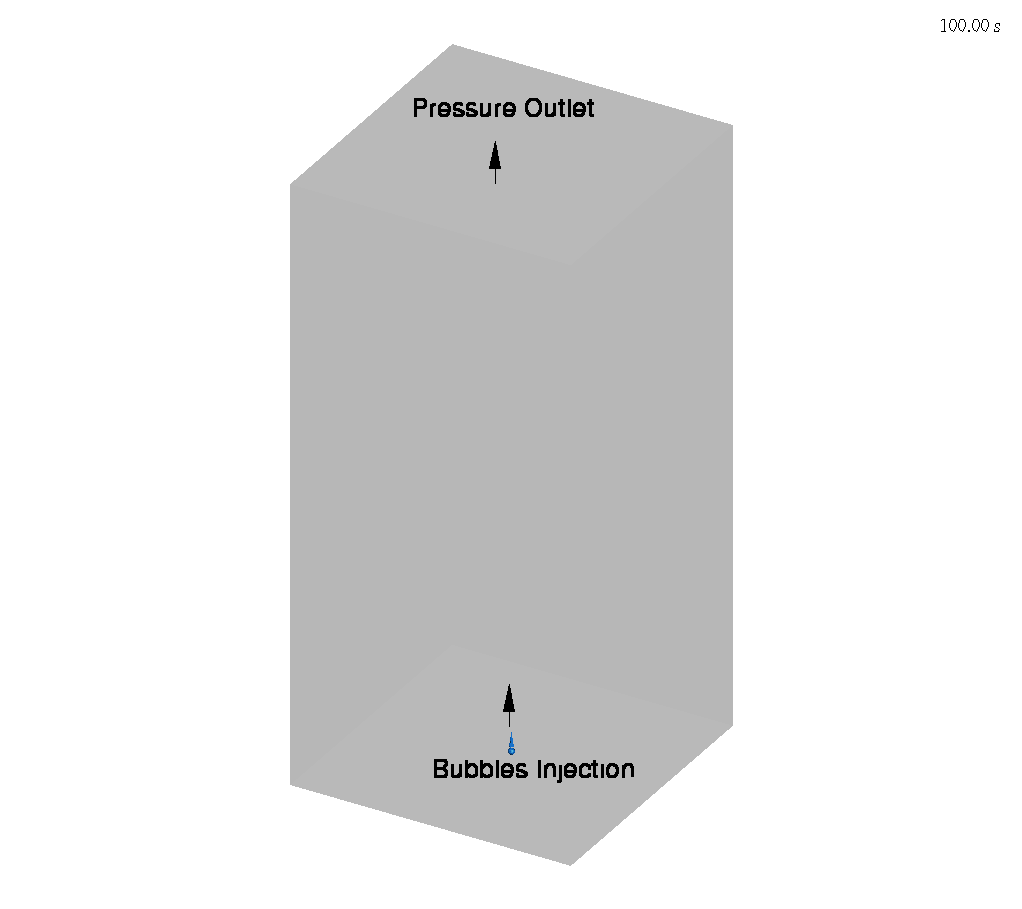
Figure 1: Argon-Fe Molten metal bubble column reactor
Results and Discussion
Figure 2 shows an animation of Ar bubbles rising up in the reactor. The bubbles are sized and colored based on their diameter. Coalescence of bubbles is observed as they move up the high-temperature molten Fe. Breakup due to shear is also observed near the injection nozzle.
Figures 3 and 4 show a comparison of the mean bubble diameter and drag coefficient, respectively, between the present Barracuda simulations and experimental and other volume of fluid (VOF) model-based CFD simulation results. To enable this comparison, Barracuda simulations were run for 5 different Ar bubble injection volumetric flow rates, ranging from 2.5 to 44 mm3/sec. The simulations were run for 100 seconds, and the mean diameter of the bubbles was calculated by taking an arithmetic average of the diameter of the computational particles or clouds tracked in the reactor at a given time. This process was repeated overall several time intervals to obtain a temporal average of the bubble diameter. The obtained bubble diameter was then used to calculate the drag coefficient. Both the mean bubble diameter and drag coefficient results obtained from Barracuda compare well with both experimental and other simulation results. It is worth noting that these Barracuda simulations were obtained on grid count of around 10,000 cells and the simulations were run for 100 seconds of physical run time compared to the VOF simulations by Ngo. et. al’ 2023 which had more than 5 million cells and were simulated for a physical run time of 3 seconds.
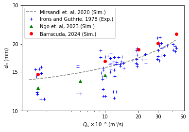
Fig 3: Comparison of mean bubble diameter with experimental and simulation results
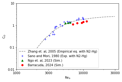
Fig 4: Comparison of drag coefficient with experimental and simulation results
Modeling Instructions
Molten Metal Bubble Column Reactor Simulation Setup
The user is expected to have already gone through basic Barracuda training, Barracuda Virtual Reactor New User Training | CPFD Software (cpfd-software.com).
- Download the support files provided along with this post.
- Unzip the support file and place it in the working directory set up for this MMBCR project.
- Open a new Barracuda session.
- From the File menu, choose Open Project. Navigate to the working directory and select mmbcr.prj.
The project file has already been set up with the appropriate
- Grid.
- Base Materials.
- Bubbles.
- Initial Conditions
- Fluid ICs.
- Particle Species.
- Boundary Conditions
- Pressure BCs.
- Flow BCs.
Some of the key highlights of the simulation setup are described in more detail below
Particles & Bubbles
In the Particles & Bubbles setup, two key inputs for this model are the Coalescence factor and the Maximum bubble size listed under Bubble Coalescence & Breakup. Figure 5 shows the values used in the present Barracuda simulation setup. The user needs to cap the bubble size growth by providing a good estimate for the Maximum bubble size input in the MMBCR setup. This value can be obtained from experimental data or theoretical correlations in the literature. In the current work, this value was estimated based on the work of Irons and Guthrie’ 1978 and Ngo et. al’ 2023. The other important parameter that the user needs to provide as input is the Coalescence factor. The coalescence factor is used by the solver in calculating a probability of coalescence, which is a function of the bubble diameter, bubble Sauter mean diameter of the cell, relative velocity between the bubbles, bubble volume fraction, turbulent dissipation rate, and the probability of breakup, which in turn is a function of bubble diameter, liquid surface tension and density, and turbulent dissipation rate. In the present work, the coalescence factor was tuned for the case with a flow rate equal to 2.5 mm3/sec such that the mean bubble diameter and drag coefficient results matched the results of Irons and Guthrie’ 1978 and Ngo et. al’ 2023. Then this tuned value of the coalescence factor was used for all remaining flow rate cases shown in Figures 3 and 4. The user can take a similar approach in tuning the coalescence factor with some known measurement data to set up different types of molten metal bubble column reactor simulations in Barracuda.
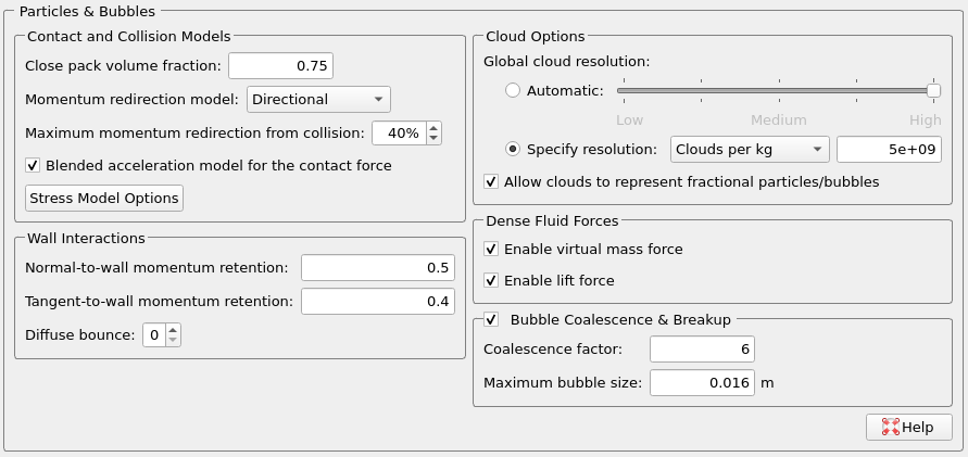
Fig 5: Particles and Bubbles setup in the present MMBCR simulation setup
Particles & Bubbles Species Manager
Under Particles & Bubbles the user needs to set up the argon bubbles species in the Particles and Bubbles Species Manager. In the current simulation, a constant bubble size value of 12 mm is provided as input in the Bubble Species Editor (Figure 6). At the inlet injection BC, the solver uses the input given in the Bubble Species Editor to inject bubbles of 12 mm in size. Since the bubble coalescence and breakup model is turned on, the injected bubbles can then either grow or break up as they advect upwards in the reactor. The bubble size distribution in the reactor is hence a function of the initial bubble size injected at the inlet of the reactor. The initial bubble size can be correlated with the inlet nozzle diameter based on the work of Islam et. al ‘ 2015. Figure 7 shows the relationship between bubble departure diameter and nozzle diameter, with a linear fit. This relationship is used to estimate the initial bubble size at the inlet injection BC in this work.
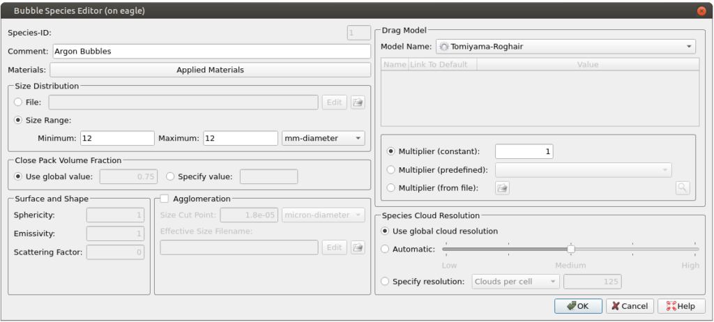
Fig 6: Bubbles species editor showing the initial bubble size injected at the inlet injection BC
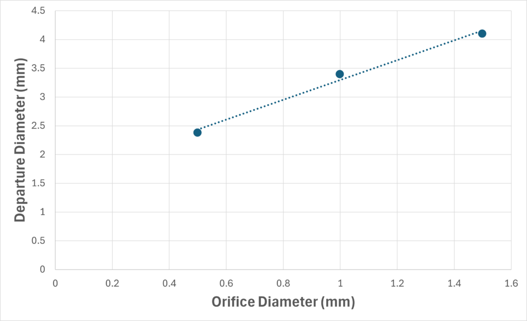
Fig 7: Relationship between Bubble departure diameter and Orifice diameter. The dotted line shows the linear fit. Data taken from Islam et. al ‘ 2015.
Time Controls
- Enter 0.001 secs for Time Step and 100 secs for End Time.
- Put 5 secs for the Restart Interval.
Visualization Data
- Enter 0.1 secs for Output file interval.
- Select the Visualization Data for post processing as shown in Figure 8.
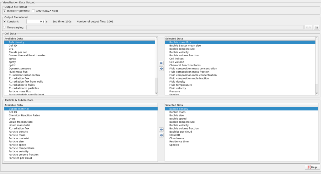
Fig 8: Visualization data
Run
- Click on Run and then click on Run Solver.
- Select GPU Parallel if you have the required GPU parallel license.
Post Processing in Tecplot
The user is assumed to have gone through basic Tecplot training, Getting Started With Tecplot For Barracuda® | CPFD Software (cpfd-software.com). So, only a few brief steps for post-processing the animation shown in Figure 2 are explained below.
- In the Barracuda GUI, click on Post-Run and then click on View Results.
- Click Ok for the information pop-up saying “Unable to find variable Particle volume fraction“.
- From the Quick Macro Panel, double click on Bubbles: Size.
- Select Zone Style and navigate to the Scatter tab
- Change the Symbol Shape to a sphere by right-clicking on the point option and selecting a sphere.
- Right-click on the default 0.15% option under the Scatter Size option.
- Pick the Select variable option to open the Scatter Size/Font dialogue box.
- Under the Scatter-size variable drop-down menu, select Bubble size.
- Under the Size multiplier option, enter 1e-7 for Grid units/magnitude.
- Click close to close the Scatter Size/Font dialogue box.
- Again, right-click on the default 0.15% option under the Scatter Size option and select By 40: Bubble size. This will scale the plotted bubbles by their size
- Close the Zone Style dialogue box.
- Click on settings beside Contour to open up the Contour & Multi-Coloring Details window.
- Click on the Set Levels and set the Minimum level to 5000, the Maximum level to 16000, and the Number of levels to 12.
- Click on the Close button to close the Contour & Multi-Coloring Details window.
- Click on the File –> Load Barracuda Data option and select All under the Tecplot Files to load option. This will load all Tecplot files at all different time steps. Click close to close the Load Barracuda Data dialogue box.
- Save the animation file by clicking on the gear symbol icon next to Solution time.
- Click on the Export to file option by hovering the mouse over the icon that looks like photo film.
- Leave the default Export format to MP4. Click Ok and provide a name to the animation file to save it in your working directory.
This concludes the description of the simulation setup process for Application Model: Bubble hydrodynamics in molten metal bubble column reactors.
References
Irons, G. A., & Guthrie, R. I. L. (1978). Bubble formation at nozzles in pig iron. Metallurgical Transactions B, 9, 101-110.
SANO, M., & MORI, K. (1980). Size of bubbles in energetic gas injection into liquid metal. Transactions of the Iron and Steel Institute of Japan, 20(10), 675-681.
Ngo, S. I., Lim, Y. I., Kwon, H. M., & Lee, U. D. (2023). Hydrodynamics of molten-metal bubble columns in the near-bubbling field using volume of fluid computational fluid dynamics. Chemical Engineering Journal, 454, 140073.
Islam, M. T., Ganesan, P. B., Sahu, J. N., & Sandaran, S. C. (2015). Effect of orifice size and bond number on bubble formation characteristics: A CFD study. The Canadian Journal of Chemical Engineering, 93(10), 1869-1879.