
Introduction
While fossil fuels continue to serve as the primary global energy source, developing carbon capture technology is essential for making their use more environmentally sustainable. A major hurdle, however, is the difficulty and energy cost of isolating carbon dioxide from nitrogen in combustion exhaust. Chemical looping combustion (CLC) offers a promising alternative, potentially enabling fuel combustion that yields pure carbon dioxide with far greater energy efficiency. A CLC system utilizes a solid oxygen carrier to keep the oxygen in air separate from the fuel source. The two exhaust gases, mainly carbon dioxide and water as well as nitrogen and oxygen, are able to be disposed of easily. Figure 1 shows a diagram of the CLC process which consists of metal oxidation in the air reactor which is then separated and transported to the fuel reactor. This metal oxide is reduced by the fuel in the fuel reactor and then separated and transported back to the air reactor.
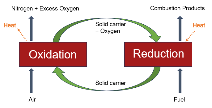
Figure 1. Diagram of CLC process
Model Definition
This Barracuda Virtual Reactor application model is based on the work of Parker (2014) with model geometry, flow conditions, and kinetics coming from that reference. The CLC system geometry – consisting of two reactors, a cyclone, a loop seal, and an L-valve – was provided by the National Energy Technology Laboratory along with operating conditions and property data for ilmenite, the solid oxygen carrier. Figure 2 shows the model reactor geometry. The grid generated for the domain consisted of approximately 168,600 real cells. The simulation was run for a total of 50 seconds. Table 1 shows the gas flow rates in the model. A small amount of coal is introduced at 0.37 g/s.
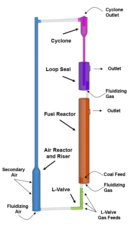
Figure 2. Schematic of CLC system
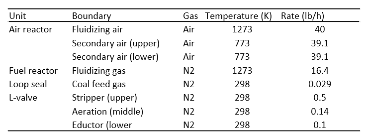
Figure 3. CLC operating conditions
The boundary conditions are shown in Figure 4.
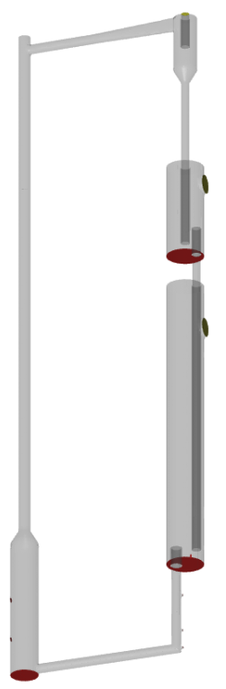
Figure 4. Boundary conditions for CLC simulation
The reaction kinetics shown below and ilmenite particle composition implemented in the model are based on the work of Abed et al. (2011).
$$ \textbf{Oxidation:} \quad 4FeO + O_2 \rightarrow 2Fe_2O_3 $$ \begin{align} \frac{dn_{Fe_2O_3}}{dt} = 2.776 \exp\left(\frac{-3.06712\times10^3}{T}\right) \left(m_{FeO}\right)^{2/3} \left(m_p\right)^{1/3} [O_2] \end{align}
$$ \textbf{CH$_4$ reduction:} \quad 4Fe_2O_3 + CH_4 \rightarrow 8FeO + CO_2 + 2H_2O $$ \begin{align} \frac{dn_{FeO}}{dt} = 8.957\times10^4 \exp\left(\frac{-1.62617\times10^4}{T}\right) \left(m_{Fe_2O_3}\right)^{2/3} \left(m_p\right)^{1/3} [CH_4] \end{align}
$$ \textbf{H$_2$ reduction:} \quad Fe_2O_3 + H_2 \rightarrow 2FeO + H_2O $$ \begin{align} \frac{dn_{FeO}}{dt} = 142.153 \exp\left(\frac{-7.81814\times10^3}{T}\right) \left(m_{Fe_2O_3}\right)^{2/3} \left(m_p\right)^{1/3} [H_2] \end{align}
$$ \textbf{CO reduction:} \quad Fe_2O_3 + CO \rightarrow 2FeO + CO_2 $$ \begin{align} \frac{dn_{FeO}}{dt} = 229.279 \exp\left(\frac{-9.70652\times10^3}{T}\right) \left(m_{Fe_2O_3}\right)^{2/3} \left(m_p\right)^{1/3} [CO]^{0.8} \end{align}
The gasification and water-gas shift kinetics shown below are based on the work of Syamlal and Bisset (1992).
$$ \textbf{Steam gasification:} \quad C(s) + H_2O \iff CO + H_2 $$ \begin{align} r_{forward} &= 6.36 \, T m_c \exp\left(\frac{-22645K}{T}\right) [H_2O] \\ r_{backward} &= 5.128\times10^{-4} T^2 m_c \exp\left(\frac{-6319K}{T} – 17.29\right) [H_2][CO] \end{align}
$$ \textbf{CO$_2$ gasification:} \quad C(s) + CO_2 \iff 2CO $$ \begin{align} r_{forward} &= 6.36 \, T m_c \exp\left(\frac{-22645K}{T}\right) [CO_2] \\ r_{backward} &= 5.128\times10^{-4} T^2 m_c \exp\left(\frac{-6319K}{T} – 17.29\right) [CO_2] \end{align}
$$ \textbf{Water-gas shift:} \quad CO + H_2O \iff CO_2 + H_2 $$ \begin{align} r_{forward} &= 1.31706\times10^{-5} p^{1.504} T^2 m_{ash} \exp\left(\frac{-8417.8K}{T} – 8.91\right) [CO][H_2O] \\ r_{backward} &= 1.31706\times10^{-5} p^{1.504} T^2 m_{ash} \exp\left(\frac{-12373.5K}{T} – 5.279\right) [CO_2][H_2] \end{align}
Results and Discussion
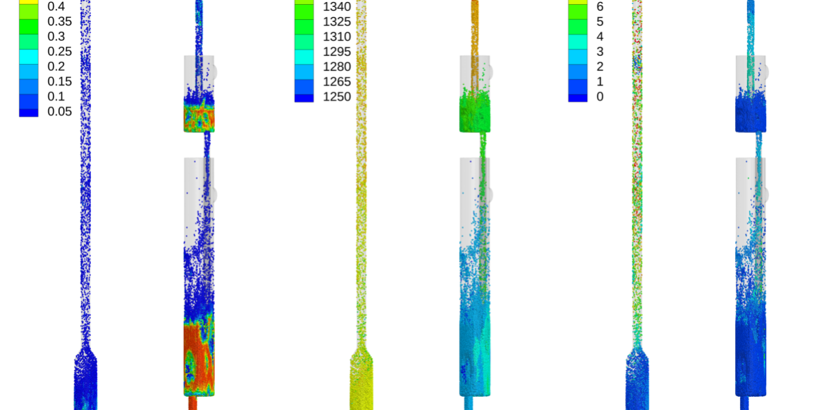
The following Tecplot images show results from the Barracuda Virtual Reactor simulation. A Tecplot for Barracuda layout file is included in the downloadable support file to reproduce these views. Figure 5 shows views of particle properties at t = 50 s. The particle volume fraction view illustrates the ability of Barracuda Virtual Reactor to simulate the full range of particle loadings from dilute to dense. This is a distinct advantage of the MP-PIC method compared to the two-fluid method. The particle temperature view highlights the fact that Virtual Reactor has tight coupling between the hydrodynamics, thermal calculations, and chemical reaction calculations. Oxidation in the air reactor is exothermic, leading to increased particle and fluid temperature. Conversely, reduction in the fuel reactor is endothermic and the particles and fluid cool down in that vessel. The particle speed view shows that particles are moving at high velocity in the riser and into the cyclone. The particles speed is relatively low in the bubbling fluidized bed vessels, as expected.
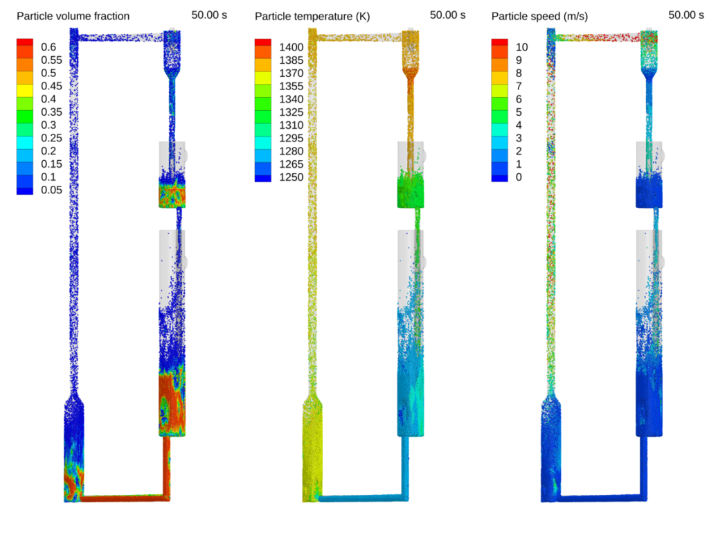
Figure 5. Particle volume fraction, temperature, and speed predicted by the Virtual Reactor simulation
Figure 6 shows views specifically related to chemistry in the CLC system. Barracuda Virtual Reactor calculates and tracks the mass fraction of all materials on every cloud in the simulation, and each particle’s composition can change due to chemical reactions. Particles enter the air reactor and undergo oxidation according to the chemical reactions listed above. FeO is converted to Fe2O3 during the oxidation reaction, and Virtual Reactor calculates the change in discrete particle mass fraction of Fe2O3 and the rate at which the reaction proceeds. The discrete reaction rate is expressed in terms of consumption of FeO; based on the sign convention used, red particles have the fastest negative reaction rates indicating the fastest rate of oxidation.
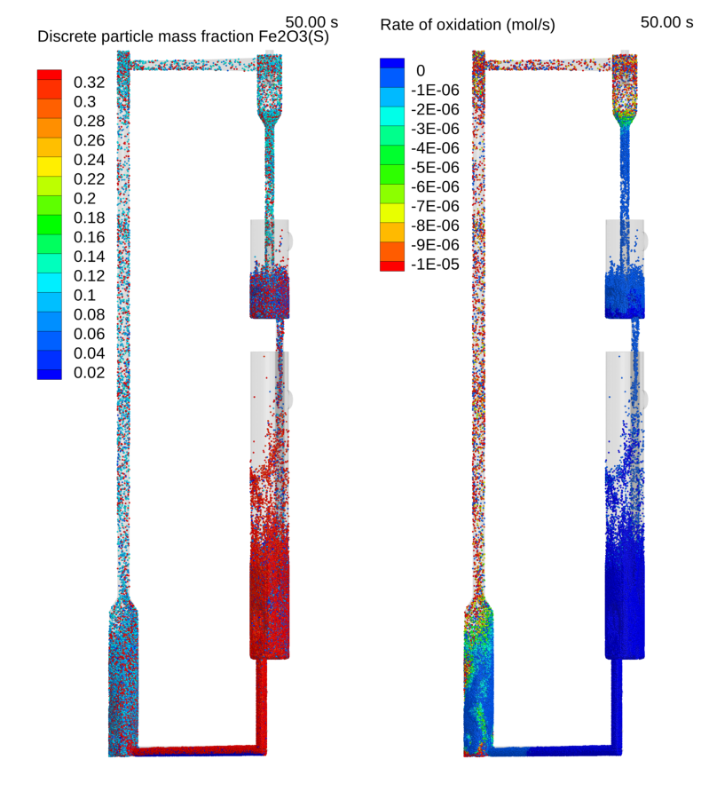
Figure 6. Particle mass fraction of Fe2O3 and rate of oxidation predicted by the Virtual Reactor simulation
In addition to tracking detailed information about particle composition, Barracuda Virtual Reactor also calculates the concentration of every gas species in the simulation in every cell at every time step. Figure 7 shows iso-surfaces of O2, CO2, and H2O mole fractions throughout the domain. Iso-surfaces are a very useful visualization technique to understand where each gas species is present throughout the system. The view of O2 mole fraction shows that the configuration of the CLC system is quite effective at preventing oxygen from entering the loop seal and fuel reactor. Likewise, CO2 is isolated to the fuel reactor and does not reach the air reactor, resulting in the possibility for highly optimized CO2 capture with downstream processing of the gas exiting the top of the fuel reactor. H2O is also effectively isolated to the fuel reactor, and its concentration is largely dictated by the equilibrium of the water-gas shift (WGS) reaction.
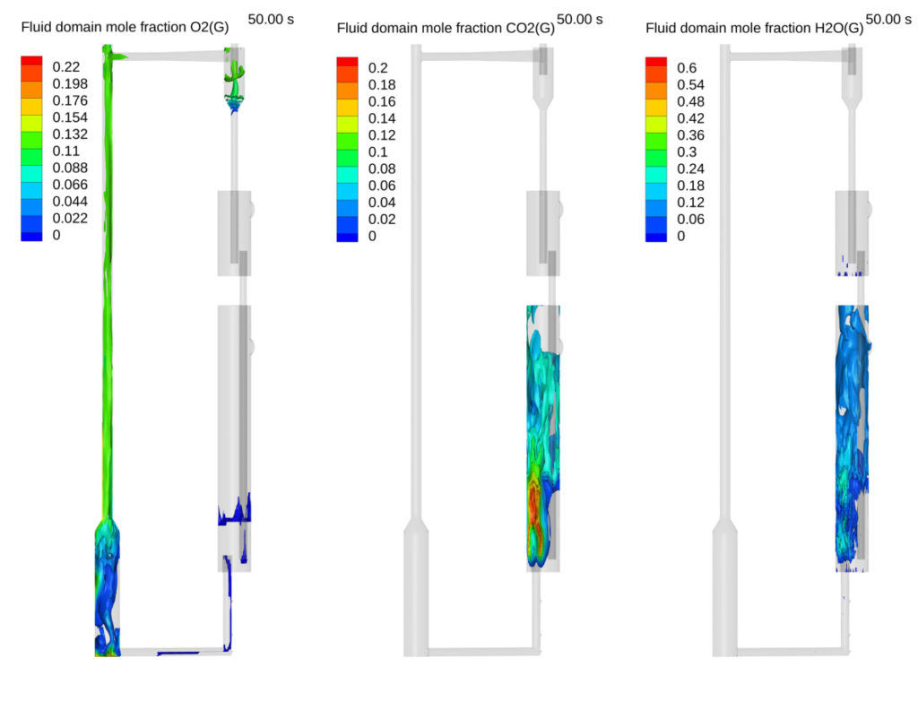
Figure 7. Fluid domain mole fraction of O2, CO2, and H2O predicted by the Virtual Reactor simulation
Modeling Instructions
Chemical Looping Combustion (CLC) Barracuda CFD Simulation Setup
The user is expected to have already gone through basic Barracuda training, Barracuda Virtual Reactor New User Training | CPFD Software (cpfd-software.com).
- Download the support file provided along with this post.
- Unzip the support file and place it in the working directory set up for this CLC project.
- Open a new Barracuda session.
- From the File menu, choose Open Project. Navigate to the working directory and select coal_clc.prj.
The project file has already been set up with the appropriate
- Grid.
- Base Materials.
- Initial Conditions.
- Fluid ICs.
- Particle Species.
- Boundary Conditions.
- Pressure BCs.
- Flow BCs.
Some of the key highlights of the simulation setup are described in more detail below
Time Controls
- Enter 0.001 secs for Time Step and 50 secs for End Time.
- Enter 20 secs for the Restart Interval.
Visualization Data
- Enter 0.2 secs for the Output file interval.
- Select the Visualization Data for post-processing as shown in Figure 8.
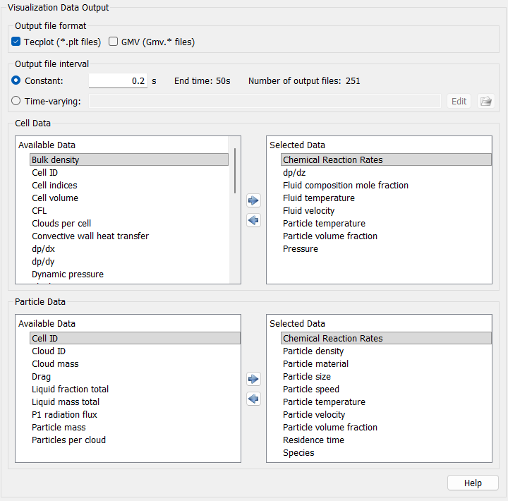
Figure 8: Visualization data selected for post-processing
Run
- Click on Run and then click on Run Solver.
- Select GPU Parallel if you have the required GPU parallel license.
Post-Processing in Tecplot
The user is assumed to have gone through basic Tecplot training, Getting Started With Tecplot For Barracuda® | CPFD Software (cpfd-software.com). Only a few brief steps for post-processing the results are explained.
To reproduce the images shown in Figure 5-7, use the layout file Fig5-Fig6-Fig7.lay provided in the zipped support file. To load the layout file into Tecplot from the Barracuda GUI:
- Navigate down to Post-Run in the project tree and select either View Results or Launch Tecplot tab.
- In the newly opened Tecplot window, select File –> Load Barracuda Data –> Load Layout, navigate to the directory where the support file was unzipped and saved, and select Fig5-Fig6-Fig7.lay and click Open. This should then reproduce the view shown in the figures.
This concludes the description of the Application Model: Coal Chemical Looping Combustion (CLC).
References
Parker, J. M. (2014). CFD model for the simulation of chemical looping combustion. Powder Technology, 265, 47–53.
Abad, A., Adanez, J., Cuadrat, A., Garcia-Labiano, F., Gayan, P., & de Diego, L. (2011). Kinetics of redox reaction of ilmenite for chemical-looping combustion. Chemical Engineering Science, 66(4), 689–702.
Syamlal, M., & Bisset, L. (1992). METC gasifier advanced simulation (MGAS) model (Technical Note No. DOE/METC-92/4108). U.S. Department of Energy.