Introduction
Hydraulic fracturing has had a profound impact on the energy industry since its conception and adoption in the 1960s and the revolution of shale fracking. Hydraulic fracking drives 75% of natural gas production and 48% of oil production in an $18.8 billion industry [3], in which over 95% of new wells in the U.S. use hydraulic fracturing [1].In modern fracking operations, vertical wells are drilled to reach hydrocarbon-bearing shale rock formations. Then, horizontal sections are extended laterally from the main vertical well, spanning the length of the shale reservoir to maximize hydrocarbon exposure. This hybrid drilling methodology developed by George Mitchell in the late 1990’s was responsible for the massive increase in shale fracking by the early 2000s. Pipes are inserted into the wellbore, and cement is poured around the pipes, stabilizing the well. Next, perforations are made in the surrounding rock formation, and high-pressure fracturing fluid is pumped into the well. Fracturing fluid (typically water with some friction reducers), known as slick water, is pumped at high pressure exceeding the tensile strength of the rock itself, causing cracks to form in the rock formation, increasing the surface area through which hydrocarbons can flow out back into the wellbore. After fractures are formed, proppants are introduced into the fracturing fluid stream. Proppants are incredibly important in fracking operations as they physically hold cracks open once the fluid pressure is reduced. The proppants provide a semi-permeable pathway for hydrocarbons to travel through and exit to the wellbore. A key consideration and area of importance in research is achieving a good distribution of proppants throughout the fracture, as well as a good material for propping. 20-50% increases in gas productivity from a well can be expected with optimization of proppants alone, and understanding how the proppants settle across a fracture and what factors influence this phenomenon is key to fracking optimization. A key resource in understanding proppant transport inside fractures has become CFD, as solvers are becoming more and more capable of accurately modeling the particle motion. The goal of this application model is to demonstrate Barracuda’s capability in modeling this process.
Model Definition
This application model exemplifies the usage of an incompressible flow simulation in Barracuda stemming from the experimental work of Mao et al, 2021 [4]. The experimental system is designed to represent a mock hydraulic fracture with dimensions: 48″ x 12″ x 0.5″. There are three inlets to the fracture and two outlets, with the three inlets spaced 3 inches from one another and a central inlet in the middle of the side wall. The two outlets include one at the same level as the top inlet on the opposite side, and a top outlet. The model geometry used in Barracuda is shown below (Figure 1).
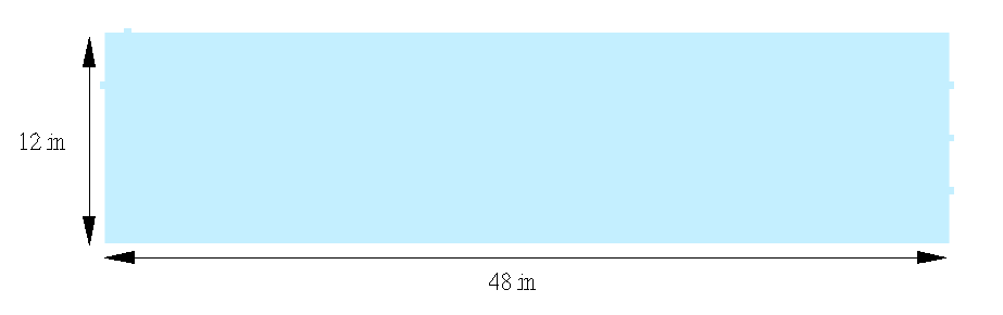
Figure 1: Fracture Channel Geometry In Barracuda
During the simulation, a slurry of frac-sand and slick water is fed through the three inlets at a combined flow rate of 6 gallons per minute, assuming the concentration of sand is 1.7 ppg. Frac-sand of size 40/70 mesh is chosen for this simulation as roughly 90% of proppant usage tends to be sand-based, with a total of 95 million tons of it being produced in 2022 alone. 40/70 mesh indicates that 90% of sand particles in the mixture must be within a size range of 212 microns to 425 microns, and the specific PSD used is included in the project file. The simulation is run for 40 seconds, and over time, the bed height and distribution of sand are of key interest and importance. A custom non-Newtonian drag model, which will be discussed further in this post was used to model the hydrodynamics of slick water, a shear-thinning fluid that is used in industry. No reactions are specified in this system, and no heat transfer is modeled as the base materials do not react and evolve any heat. A single flow BC is defined over all three inlets, and two pressure BC’s are defined at the outlets with particle outflow allowed (negligible outflow). Finally, the system operates at atmospheric pressure and room temperature.
Non-Newtonian Drag Model
In Barracuda, drag models are all defined relative to the Stokes drag law, which explains the drag force acting upon a small spherical particle moving through viscous fluids at low Reynolds numbers. Of course, this case is not at all universally applicable, and 13 standard drag models are available to choose from in Barracuda. For this simulation, a modified version of the Beetstra drag model developed by Chhabra in 1990 [2] was used in order to account for the non-Newtonian shear thinning nature of slick water being used as fracking fluid. The Chhabra drag model was specified using a user-defined drag expression and is shown below in Figure 2. Drag expressions are related to Stokes’ law. To define this drag model for slick water, several power law-based parameters were adopted.
For a Newtonian fluid, the shear stress experienced is linearly proportionate to the rate of shear, where \( \tau \) is the shear stress (in Pa), \( \mu \) is the dynamic viscosity (in Pa·s), and \( \dot{\gamma} \) is the shear rate (in s\(^{-1}\)).
\begin{equation}
\tau = \mu \, \dot{\gamma}
\end{equation}
For non-Newtonian fluids, however, the relationship between shear stress and shear rate is non-linear, and it becomes beneficial to re-write the stress relationship in a different manner. Shear rate \( \dot{\gamma} \) is defined as the velocity gradient perpendicular to the direction of flow. For flow in the \( x \)-direction with a velocity field \( u(y) \), the shear rate is given by:
\begin{equation}
\dot{\gamma} = \frac{du}{dy}
\end{equation}
In many non-Newtonian fluids, the shear stress due to viscosity can be modeled more specifically as a power law model:
\begin{equation}
\tau_{xy} = K \left( \frac{du}{dy} \right)^n
\end{equation}
where \( \tau_{xy} \) is the shear stress, \( K \) is the consistency index (units Pa·s\(^n\)), \( n \) is the flow behavior index (dimensionless), and \( \frac{du}{dy} \) is the shear rate.
To ensure that the shear stress \( \tau_{xy} \) always has the same sign as \( \frac{du}{dy} \), this expression is often rewritten to preserve sign information explicitly:
\begin{equation}
\tau_{xy} = K \left| \frac{du}{dy} \right|^{n-1} \frac{du}{dy}
\end{equation}
From this, we can define the effective viscosity \( \mu_{\text{eff}} \) as:
\begin{equation}
\mu_{\text{eff}}\ = K \left| \frac{du}{dy} \right|^{n-1}
\end{equation}
So the shear stress can be written in a Newtonian-like form using the apparent viscosity:
\begin{equation}
\tau_{xy} = \mu_{\text{eff}}\ \frac{du}{dy}
\end{equation}
This expression shows that the apparent viscosity depends on the shear rate. When \( n = 1 \), \( \mu_{\text{eff}} = K \), and the fluid behaves as a Newtonian fluid with constant viscosity.
A characteristic shear rate around a spherical particle can be approximated by:
\begin{equation}
\dot{\gamma} = \frac{|u_f – u_s|}{d_p}
\end{equation}
Substituting this characteristic shear rate into the effective viscosity expression yields:
\begin{equation}
\mu_{\text{eff}} = K\left(\frac{|u_f – u_s|}{d_p}\right)^{n-1}
\end{equation}
The classical particle Reynolds number for a spherical particle in a Newtonian fluid is defined as:
\begin{equation}
Re_p = \frac{\rho_f d_p |u_f – u_s|}{\mu_f}
\end{equation}
Replacing the Newtonian viscosity in the Reynolds number definition with the effective viscosity, we have:
\begin{align}
Re_{p,n} &= \frac{\rho_f d_p |u_f – u_s|}{\mu_{\text{eff}}} \\
&= \frac{\rho_f d_p |u_f – u_s|}{K\left(\frac{|u_f – u_s|}{d_p}\right)^{n-1}} \\
&= \frac{\rho_f d_p^n |u_f – u_s|^{2-n}}{K}
\end{align}
Therefore, the modified Reynolds number for a Power-law non-Newtonian fluid is:
\begin{equation}
Re_{p,n} = \frac{\rho_f d_p^n |u_f – u_s|^{2-n}}{K}
\end{equation}
Additionally, a dimensionless viscosity ratio can compare the non-Newtonian value to that of a reference Newtonian fluid. The dimensionless viscosity ratio is defined as:
\begin{align}
\frac{\mu_{\text{eff}}}{\mu_f} &= \frac{K\left(\frac{|u_f – u_s|}{d_p}\right)^{n-1}}{\mu_f} \\
&= \frac{K|u_f – u_s|^{n-1} d_p^{1-n}}{\mu_f}
\end{align}
Model Setup
The model provided in the support file includes the following, already set up properly:
- Gridded Geometry
- Base Materials and Properties
- Particle Species
- Boundary Conditions
- Output Visualization Specification
As discussed previously, this model exemplifies the usage of a non-Newtonian drag model. A key consideration here is that while drag forces are calculated for a non-Newtonian fluid, the solver models the fluid as Newtonian. This is an area where developmental efforts are underway. In Barracuda, several pre-defined drag models are available for usage and specification. To select an appropriate drag model, follow the proceeding instructions.
- Under Particles and Bubbles in the project tree, navigate to the Drag Models section.
- Here, 13 predefined drag models are provided; users can define their own if desired.
- To add a user-defined drag model, simply select Add and enter the expression as desired. For this simulation, the drag model is entered as shown in Figure 2 below, based on the derivations in the above section.
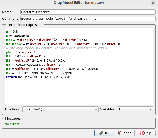
Figure 2: User-Defined Drag Model for Non-Newtonian Fluids
.
Results and Discussion
Using a 40/70 mesh frac-sand PSD [5], results for the simulation are shown below. Initially, a slurry of frac-sand and slick water is pumped into the fracture channel and falls closer to the inlet side of the fracture, but over time, the bed height increases and a more dune-like structure is achieved. As seen in Figure 3, at ten seconds, proppant begins to settle and has yet to span the length of the fracture. At 20 seconds, the proppant has traveled further into the fracture, and a dune of sand begins to accumulate as the bed height begins to increase towards the entrance. Finally, at 40 seconds, the proppant bed spans the length of the fracture, and a full dune distribution is seen in the channel. As proppant travels further through the channel, it is clear in the animation shown in Figure 4 that sand begins to settle down more immediately, leading to the increased height towards the injection points. This is commonly referred to as a heel-skewed distribution, which is undesirable in fracking applications. Mitigation of this phenomenon provides a more even coverage of fractures, ensuring that sections near the toe-end do not close.
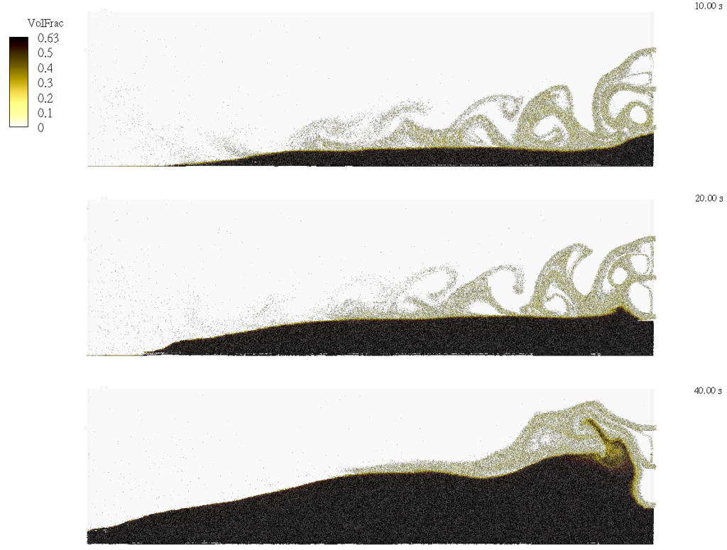
Figure 3: Proppant Bed Height in Fracture Channel at 10, 20, and 40 seconds.
Figure 4: Animation showing proppant volume fraction, velocity, and age.
Proppant Transport in slick water is controlled by fluidization and sedimentation. In regions of fluidization, proppants are carried by turbulent fluid near the inlet and eventually settle further away in the sedimentation zone to form the proppant bed. The zone in between the two experiences erosion of the bed in which proppant is “washed out” further down the dune. These behaviors are further visualized in Figure 5, which displays the simulated proppant velocity. As seen below, the darker blue particles have zero velocity and have settled in the bed. Slightly above this layer is the erosion boundary, in which particles at intermediate velocities slide down the bed and eventually settle. Above this is a region of fluidization where particles are carried in at higher velocities, around 1 m/s. There is a stark contrast between the sedimentation and fluidization zones in terms of velocity, and Barracuda does well to capture these behaviors.
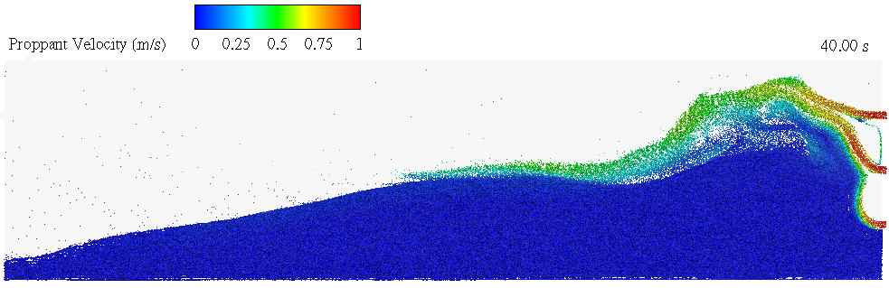
Figure 5: Proppant Velocity in Fracture at 40 Seconds.
Barracuda also captures the settling behavior of proppants with respect to time. In Figure 6, the age of proppant is shown to decrease with bed height, indicating that new proppants are added to the bed, increasing its height, while older proppants remain settled, forming layers. The older red proppants settle into the sedimentation layer early on, while newer blue proppants are carried in the fluidization layer and travel across the proppant bed upon injection. A layer in between the two layers is comprised of intermediate proppants that settle on top of the oldest ones, not fully reaching the end of the fracture channel as the bed height begins to increase and the distribution becomes more heel-skewed with time.
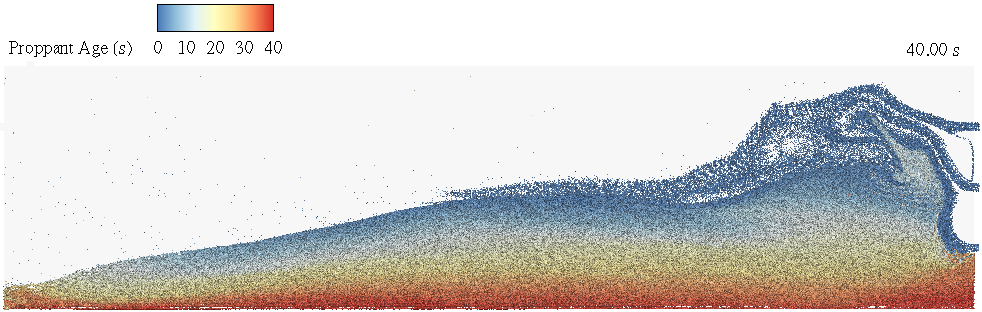
Figure 6: Proppant Age in Fracture at 40 Seconds.
A major factor that influences the distribution of proppant is the particle size distribution (PSD), and no definite particle size distribution was stated in the experimental work on which this modeling is based. The size distribution was said to be of 40/70 mesh, meaning that 90% of the particles had to fall within a range of 212 to 425 microns in diameter. Due to the unavailability of the experimental PSD, an estimation was sourced from literature, and the resulting bed height comparisons at 10, 20, and 40 seconds between the experiment and the Barracuda simulation are shown below in Figure 7. While the actual maximum bed height of the experiment is not reached, the dynamics of proppant transport are captured effectively through time as seen by the steady rise to a proppant dune. The inconsistency with experimental results can be attributed mostly to a difference in PSDs. To demonstrate the size distribution’s impact on bed settling characteristics, two simulations were run using smaller and larger uniform size distributions at the limits of the 40/70 mesh size distribution (212 and 425 micron diameter). Figure 8 shows the distribution of particles in the fracture for a smaller and larger particle diameter, along with the experimental and simulation results at 40 seconds. The smaller size distribution is essentially uniform across the fracture, but packs significantly lower, whereas the larger particle distribution features a very heel-centered distribution with very few particles actually reaching the toe end of the fracture. Somewhere in between the two size ranges will yield the same results as in the experiment, and Barracuda is entirely capable of optimizing this metric.
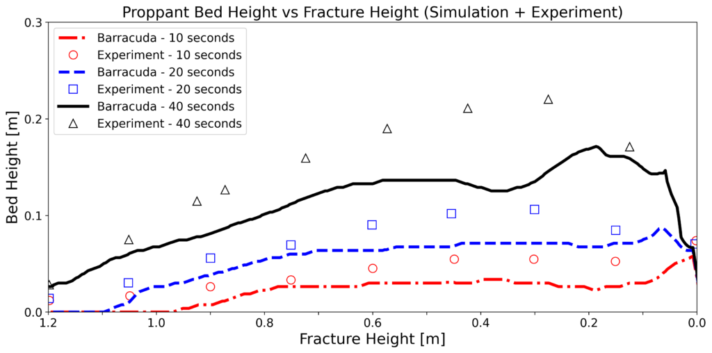
Figure 7: Proppant Bed Height Comparison Between Simulation and Experiment at 10, 20, and 40 Seconds.
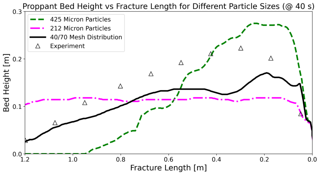
Figure 8: Settling behavior comparison between the 40/70 mesh simulation, 212 micron diameter simulation, 425 micron diameter simulation, and the experiment.
Post Processing
Download the project support file here. The user is expected to have completed Barracuda Virtual Reactor New User Training before attempting to run this application model.
Simply navigate to Run in the project tree and select Run Solver.
To reproduce the included results as seen in Figure 3, follow the instructions below:
- In the Barracuda GUI, navigate to Post-Run and select View Results.
- Load in all Barracuda data, then put the plot view into the YZ plane.
- Rotate the geometry 180 degrees using the Spherical Rotation tool.
- Ensuring that the border of the frame is selected, copy and paste the frame 2 times, and tile the frames vertically.
- Select Frame, Frame Linking, and check the option 3D Plot View, ensuring that the Apply Settings to All Frames of this Group button is selected afterwards.
- Resize the legend for the top frame by selecting it, navigating to Frame, changing the text from Frame% to Points, and changing the point value to 16. Delete the other legends by right-clicking and selecting Hide.
- Additionally, change the values in the legend by selecting Levels and Color, Set Levels, and setting 0 to 0.63 with 6 levels.
- Change the color map to CPFD Sand.
- In the same page, select the Continuous Color map distribution option and ensure that the min and max values are the same limits as the Contour Levels.
- Finally, for each frame, change the Solution time to 10, 20, and 40 seconds.
- For each frame, navigate to Zone Style, Effects, and set the Surface Translucency value for cells to 90 by right-clicking to open the drop-down menu.
- Also in Zone Style, change the Shade Color under Shade to White, and set the Scatter Symbol Shape to a Sphere of 0.10% Scatter Size.
To reproduce the results in Figure 4, follow the instructions below.
- Open a new Tecplot window per instructions 1-3 for Figure 3.
- Select Contour Options and change the variable to Particle Speed.
- Under Levels and Colors, select Modified Rainbow – Less Green.
- Also in Levels and Colors, Set Levels to 0 to 1 using 5 levels.
- Select the Continuous color map distribution method and set the min and max to 0 and 1.
- The following changes are to be made in the Legend tab of the Contour Options:
- Change the alignment to Horizontal by clicking in the Alignment dropdown menu, and uncheck the Separate color bands option.
- Set the X and Y alignment to 2.25 and 70.5, respectively.
- Under Header Text, select Use Text from the dropdown menu and type “Proppant Velocity (m/s)”, setting the font size to Points and selecting 12
- Under Zone style, follow the same procedure as in steps 11/12 of the Figure 3 instructions to change the shading to an appropriate value.
To reproduce the results in Figure 5, follow the instructions below:
- Open a new Tecplot window as directed in steps 1-3 of the Figure 3 instructions.
- Select Contour Options and change the variable to Residence Time.
- Under Levels and Colors, select Diverging Blue/Yellow/Red.
- Also in Levels and Colors, Set Levels from 0 to 40 using 7 levels.
- Select the Continuous color map distribution method and set the min and max to 0 and 40.
- Complete the same directions as in Step 6 of the Figure 4 instructions, this time changing the title to “Proppant Age (s)“.
- Under Zone Style, follow the same procedure as in the Figure 3 instructions, steps 11/12 to change the shading to an appropriate value.
References
- American Petroleum Institute. Hydraulic Fracturing: Better for the Environment and the Economy. PDF, api.org, https://www.api.org/-/media/files/oil-and-natural-gas/hydraulic-fracturing/environment-economic-benefits/api_frackingbenefits_final_.pdf
- Chhabra, R. P. “Motion of Spheres in Power Law (Viscoinelastic) Fluids at Intermediate Reynolds Numbers: A Unified Approach.” The Canadian Journal of Chemical Engineering, vol. 68, no. 3, 1990, pp. 470–476. DOI: 10.1002/cjce.5450680319.
- Everything Policy. “Fracking.” Everything Policy – Policy Briefs, 21 May 2024, www.everythingpolicy.org/policy-briefs/fracking
- Mao, Shaowen, Zhuo Zhang, Troy Chun, and Kan Wu. “Field-Scale Numerical Investigation of Proppant Transport among Multicluster Hydraulic Fractures.” SPE Journal, vol. 26, no. 1, Feb. 2021, pp. 307–323. Society of Petroleum Engineers, https://doi.org/10.2118/203834-PA.
- PropTester Inc. 40/70 Mesh Sand Lab Report. Carbo Ceramics, 17 Dec. 2020. Scribd, www.scribd.com/document/769640088/40-70-Mesh-Sand. Accessed 4 Aug. 2025.
- U.S. Environmental Protection Agency. Hydraulic Fracturing for Oil and Gas: Impacts from the Hydraulic Fracturing Water Cycle on Drinking Water Resources in the United States. EPA/600/R-16/236F, Dec. 2016. https://www.epa.gov/hfstudy.