
Introduction
Steel production currently accounts for 8% of global energy demand and 7% of global carbon dioxide emissions (Yu et al., 2021). Traditional steelmaking technologies such as basic oxygen blast furnaces involve combusting coke and other carbonaceous materials in order to provide the reducing environment for steel production, resulting in significant carbon dioxide emissions. Recent focus has turned towards the use of lower carbon technologies for steel production, specifically direct reduced iron (DRI) steel production in a shaft furnace. In this method, the iron ore materials are reacted directly with a reducing gas mixtures containing hydrogen and carbon monoxide. It has been shown that the use of a mixture of hydrogen, methane, and carbon monoxide results in the reduction of carbon dioxide emissions by 61% compared to basic oxygen blast furnace technologies. Additional replacement of the methane with hydrogen can reduce carbon dioxide emissions by 97% (Yu et al., 2021).
This application model exemplifies the setup of a moving bed, thermal, and compressible system with both volumetric and discrete reaction chemistry using Barracuda Virtual Reactor (referred to as Barracuda in the remainder of the post). It also demonstrates the usage of the user-defined rate expression feature in Barracuda. In this post, the model results are presented and compared with 2D isometric results from available literature.
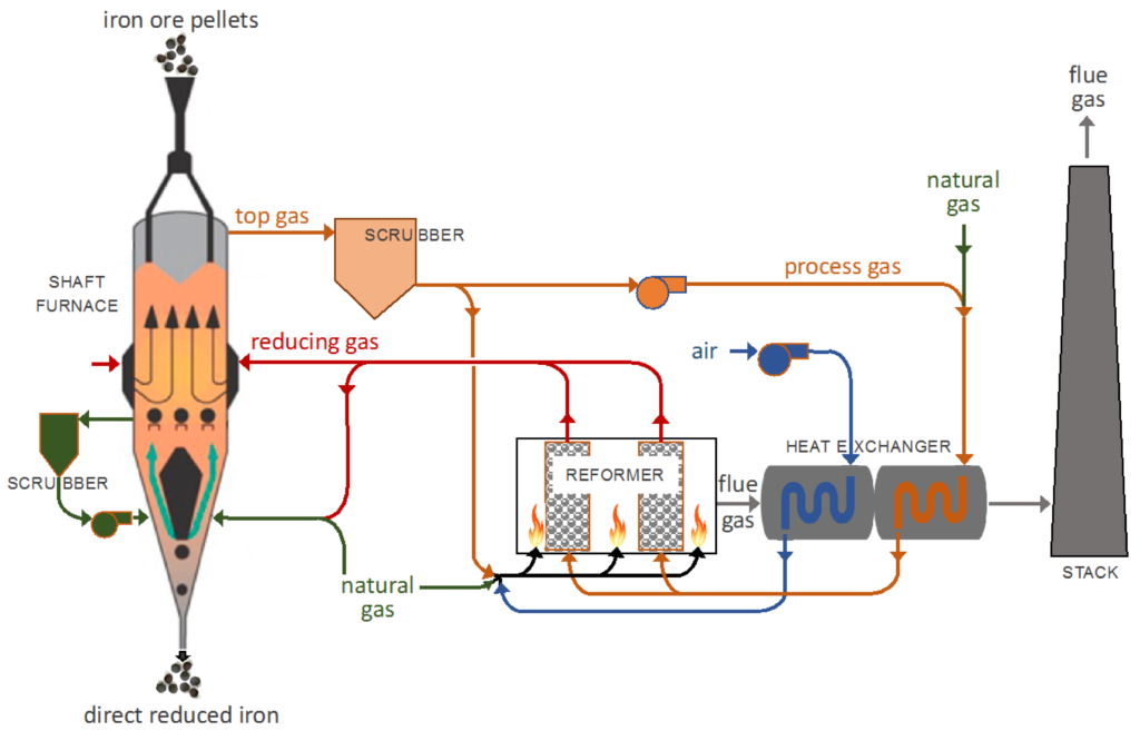
Figure 1: MIDREX process flow diagram taken from Hamadeh et al. 2018
In the MIDREX process, reduced iron is produced from iron ore using a shaft furnace. In the furnace, iron ore pellets consisting of hematite are fed in through the top of the shaft furnace where they flow countercurrent to a reducing gas mixture containing hydrogen and carbon monoxide. This gas mixture is obtained from the catalytic reforming of natural gas. The solids descend down the shaft furnace in a moving bed as they undergo reduction, and are transported to the outlet at the bottom where they are released as the reduced iron product. An additional cool natural gas stream is fed in along with a portion of the reducing gas mixture to the bottom of the vessel, which cools the product to a lower temperature and supports the solids in the moving bed. The model domain includes only the shaft furnace and not the catalytic reforming of natural gas.
Model Definition
The geometry used for this model was sourced from a paper describing the operating conditions for a MIDREX plant in Quebec, Canada (Hamadeh et al., 2018). The input data for this plant, including flow rates, compositions, and pressures, are provided in Hamadeh et al., 2018 and are used for this model setup. The smallest diameter of the vessel spans 2 m in the cooling section and the widest at 5.5 meters in the reducing section. The vessel is 25 m in height with a 15 m tall reducing section and a 10 m tall cooling section. The shaft furnace is divided into 3 different zones: the cooling zone, reducing zone, and transition zone. In the cooling zone, a low-temperature (41 °C) gas stream containing a high fraction of methane is fed in at a rate of 7.7 kg/s, which cools down the solids to a temperature of 285 °C. Per specifications described in Hamadeh et al., 2018, 10% of the cooling gas is allowed up from the cooling section into the reducing section. The flow of gas up the furnace and into the reducing section is controlled by adjusting the flow at the gas vent Flow BC. To achieve 10% flow into the reducing section, the flow rate out of the gas vent is set at 7 kg/s.
In the reducing zone, reducing gas at a temperature of 957 °C is fed in through the outer wall. The gas requires preheating to reach a suitable temperature for the operation of the furnace, primarily due to the endothermic nature of the reduction reactions involving hydrogen. While the reduction by hydrogen is an endothermic process, the reduction by carbon monoxide is a slightly exothermic process. Therefore, including a mixture of the two species enables the system to recover some of the sensible heat lost to endothermic reduction reactions. The mixture composition is taken from MIDREX input data and is the product of the catalytic reforming of natural gas.
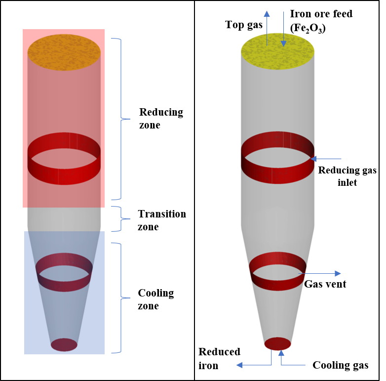
Figure 2: Shaft furnace process description
The particle species modeled include all the intermediate species involved in the three-step reduction of the iron ore, including hematite (Fe2O3), magnetite (Fe3O4), wustite (FeO), and iron (Fe). All species are defined with a uniform 15 mm particle diameter and a density of 3500 kg/m3. The remaining particle properties are functions of temperature in Barracuda. The Beetstra drag model is used to model the drag imposed one each particle species across the model. Due to the long residence times in the moving bed, the particle initial conditions are set to approximate a distribution of solids in the shaft furnace that is close to steady-state. A diagram of these Particle ICs can be seen in Figure 3. The initial particle and fluid temperature are both set at 650 °C. for all species except for the hematite (Fe2O3) which is set a lower initial temperature of 450 °C. This is intended to account for the lower temperature at which the hematite particles are fed into the top of the vessel. These particles are fed in at a temperature of -10 °C and then are rapidly heated by the hot gases flowing countercurrent to the solids. Due to the run times of this model to a steady state value, an IC file is included in the support file download link which will allow the user to run the model from IC at a solids distribution closer to steady state.
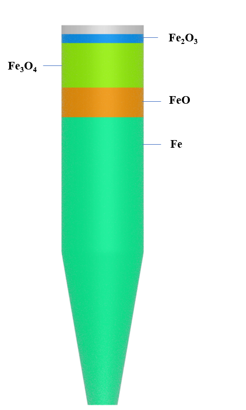
Figure 3: Particle initialization in Barracuda
Reaction Kinetics
The kinetics modeled in the shaft furnace system include both heterogeneous reactions between the particle and gas phase, which are modeled as discrete reactions, as well as gas-phase homogeneous reactions, which are modeled as stoichiometric reactions. Reactions 1-3 describe the reduction of the iron oxide by hydrogen and reactions 4-6 describe the solids reduction by carbon monoxide. Reaction 7-8 represent the carburization reactions by means of which carbon is deposited onto the particles. Reaction 9 describes the production of iron carbide (Fe3C), a key component in steel production. Finally, Reactions 10-11 are gas-phase stoichiometric reactions which include water-gas shift and the steam methane reforming reaction. The full reaction set is included below:
\[
\begin{gathered}
3Fe_2O_3 + H_2 \rightarrow 2Fe_3O_4 + H_2O \quad \text{(1)} \\[8pt]
3Fe_2O_3 + H_2 \rightarrow 2Fe_3O_4 + H_2O \quad \text{(1)} \\[8pt]
Fe_3O_4 + H_2 \rightarrow 3 FeO + H_2O \quad \text{(2)} \\[8pt]
FeO + H_2 \rightarrow Fe + H_2O \quad \text{(3)} \\[8pt]
3Fe_2O_3 + CO \rightarrow 2 Fe_3O_4 + CO_2 \quad \text{(4)} \\[8pt]
Fe_3O_4 + CO \rightarrow 3 FeO + CO_2 \quad \text{(5)} \\[8pt]
FeO + CO \rightarrow Fe + CO_2 \quad \text{(6)} \\[8pt]
2CO \leftrightarrow C + CO_2 \quad \text{(7)} \\[8pt]
CH_4 \leftrightarrow C + 2H_2 \quad \text{(8)} \\[8pt]
3Fe + 2CO \leftrightarrow Fe_3C + CO_2 \quad \text{(9)} \\[8pt]
CH_4 + H_2O \leftrightarrow CO + 3 H_2 \quad \text{(10)} \\[8pt]
CO + H_2O \leftrightarrow CO_2 + H_2 \quad \text{(11)} \\[8pt]
\end{gathered}
\]
For modeling the reduction of the iron oxide pellet by both H2 and CO (Reactions 1-6), the unreacted shrinking core model (UCSM) is used from Hara et al., 1976 and is described in detail in Immonen and Powell, 2024. This model assumes constant volume for the iron oxide pellet as the reaction progresses. In the standard UCSM model, both reaction resistances and diffusional resistances are modeled between each iron oxide layer in the pellet. For entry in Barracuda, these expressions have been simplified to include only the reaction resistances. It is also noted that the diffusional resistances described in Hara et al., 1976 have a high degree of uncertainty and were therefore neglected in this model (Hara et al., 1976).
The UCSM model described here includes the three-step reduction of iron ore. In general, the kinetic model uses the ratio of the radius of each iron oxide layer over the radius of the particle to describe the progression of the iron oxide reduction. For the Barracuda implementation, this ratio is approximated based on the mass of the iron oxide species divided by the mass of the entire particle.
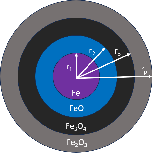
Figure 4: UCSM model iron oxide layers
The general form of the rate expression for the reduction of the solids is equal to:
\begin{gathered}
R_i = \frac{4πr_p^2}{W}\left( C_{H_2} – C_{H_2,eq} \right) \\[8pt]
\end{gathered}
where W refers to the resistance and C refers to the molar concentration of the species in units of mol / m3. The term CH2,eq refers to the equilibrium concentration of Hydrogen. For this case, we are simply considering the chemical reaction resistance so W reduces down to the expression:
\begin{gathered}
W = \frac{1}{X_i^2 \left[ k_j \left( 1+ frac{1}{K_{eq,i}} \right) \right]} \\[8pt]
\end{gathered}
X refers to the fraction of each iron oxide species that is reacted which is described by the following expression. The term M refers to the mass of the
\begin{gathered}
X_i = \left( \frac{m_{Fe_xO_y}}{m_{particle}} \right)^{\frac{2}{3}} \\[8pt]
\end{gathered}
The expression therefore becomes:
\begin{gathered}
R_i = 4πr_p^2k_j \left( 1 – \frac{m_{Fe_xO_y}}{m_{particle}} \right)^{\frac{2}{3}} \left( 1+\frac{1}{K_{eq}} \right) \left( C_{H_2} – C_{H_2,eq} \right) \\[8pt]
\end{gathered}
The rate expressions for the solids reduction are listed below (Immonen and Powell, 2024)
\[
\begin{gathered}
k_1 = 0.89124 \times exp \left( \frac{-4017.32}{T_p} \right) \quad{(1)} \\[8pt]
k_2 = 8.1241 \times exp \left( \frac{-7000.24}{T_p} \right) \quad \text{(2)} \\[8pt]
k_3 = 10.6422 \times exp \left( \frac{-6867.9}{T_p} \right) \quad \text{(3)} \\[8pt]
k_4 = 0.235706 \times exp \left( \frac{-6038}{T_p} \right) \quad \text{(4)} \\[8pt]
k_5 = 0.080849 \times exp \left( \frac{-4811.16}{T_p} \right) \quad \text{(5)} \\[8pt]
k_6 = 2.258791 \times exp \left( \frac{-7385.1}{T_p} \right) \quad \text{(6)} \\[8pt]
\end{gathered}
\]
The equilibrium constants are described below:
\[
\begin{gathered}
K_{eq,1} = exp \left( \frac{1433.37}{T_p} + 9.083 \right) \quad \text{(1)} \\[8pt]
K_{eq,2} = exp \left( \frac{-7393.9}{T_p} + 7.563\right) \quad \text{(2)} \\[8pt]
K_{eq,3} = exp \left( \frac{-2023.8}{T_p} + 1.239 \right) \quad \text{(3)} \\[8pt]
K_{eq,4} = exp \left( \frac{5128.6}{T_p} + 5.7 \right) \quad \text{(4)} \\[8pt]
K_{eq,5} = exp \left( \frac{-3132.5}{T_p} + 3.661\right) \quad \text{(5)} \\[8pt]
K_{eq,6} = exp \left( \frac{2240.6}{T_p} – 2.667 \right) \quad \text{(6)} \\[8pt]
\end{gathered}
\]
For modeling the carburization reactions (Reaction 7 and 8), kinetics were adopted from literature (Immonen and Powell, 2024). This includes the CO disproportionation reaction (Reaction 7) and the methane decomposition reaction (Reaction 8). The rate expressions for these kinetics are described below:
\[
\begin{gathered}
R_7 = V_p \left( k_{7}P_{H_2}^{0.5} + k_{7}^{‘} \right) \left( P_{CO}^2 – \frac{P_{CO_2}α_c}{K_{eq,7}} \right) \quad \text{(7)} \\[8pt]
R_8 = \frac{V_pk_8}{P_{H_2}^{0.5}} \left( P_{CH_4} – \frac{P_{H_2}^2α_c}{K_{eq,8}} \right) \quad \text{(8)} \\[8pt]
\end{gathered}
\]
The term αc refers to the carbon activity and is a function of the atomic ratio of the carbon and iron (ξ). This relationship is described here (Chipman, 1972):
\begin{gathered}
α_c = exp \left[ \frac{2300}{T} – 0.92 + \left( \frac{3860}{T} \right)ξ^{ratio} + log \left( \frac{ξ^{ratio}}{1-ξ^{ratio}} \right) \right] \\[8pt]
\end{gathered}
The carburization reactions described here only occur on metallic iron. Therefore, the rate constants are defined with a dependence on the progress of the iron oxide reduction. In the unreacted shrinking core model (USCM), the iron oxide reduction progress (F) is quantified with the following expression:
\begin{gathered}
F = 1 – \frac{1}{9}X_1 – \frac{2}{9}X_2 – \frac{2}{3}X_3 \\[8pt]
\end{gathered}
The rate constants are defined in the following manner based on the iron oxide reduction progress:
\[
\begin{gathered}
k_{7} = \begin{cases}
\text{if } F \lt 0.4 & 0 \\
\text{if } F \ge 0.4 & 1.8 \times exp \left( \frac{-27200}{RT_s} \right) \\
\end{cases} \\
k_{7}^{‘} = \begin{cases}
\text{if } F \lt 0.4 & 0 \\
\text{if } F \ge 0.4 & 2.2 \times exp \left( \frac{-8800}{RT_s} \right) \\
\end{cases} \\
k_8 = \begin{cases}
\text{if } F \lt 0.4 & 0 \\
\text{if } F \ge 0.4 & 16250 \times exp \left( \frac{-55000}{RT_s} \right) \\
\end{cases}
\end{gathered}
\]
Finally, the equilibrium constants for these reactions are included here:
\[
\begin{gathered}
K_{eq,7} = exp \left( \frac{180,030.9 – 402.82T_s + 0.00524T_s^2 – 828,509.9T_s^{-1} + 32.026T_slog(T_s)}{RT_s} \right) P_g^{-1} \\[8pt]
K_{eq,8} = exp \left( \frac{89,658.88 – 102.27T_s – 0.00428T_s^2 – 2,499,358.99T_s^{-1} + 18,000}{RT_s} \right) P_g \\[8pt]
\end{gathered}
\]
Another important reaction for steel production is iron carbide production. Due to limited kinetic data is available for this reaction, most studies to date do not distinguish between the production of carbon and iron carbide and simply represent carbon production (Hamadeh 2018). Though there is data available on the activation energy and rate constants for this reaction, these do not include dependencies on the concentration and particle properties in the manner that is described in the CO disproportionation reaction in Immmonen 2021 (Mondal, 2004). Therefore, for entry in Barracuda, the same form of the rate equation from the CO disproportionation reaction (reaction 7) was applied, with a scale ratio calculated between its rate constant and the one provided in the Mondal paper (Mondal, 2004). Taken over a temperature interval of 650 to 1250 K, this average scale ratio is equal to 6.25. Therefore, the reaction rate is described with the following expression:
\begin{gathered}
R_9 = 6.25V_pk_0 \left( P_{CO}^2 – \frac{P_{CO_2}α_c}{K_{eq,9}} \right) \quad \text{(9)} \\[8pt]
\end{gathered}
In this case, the value of k0 is taken from Mondal 2004 and is equal to 0.082.
The final two gas-phase reactions include the steam-methane reforming reaction (Reaction 10) and the water-gas shift reaction (Reaction 11). These reaction rates also have a dependency on the degree of reduction of the iron oxides. For the water-gas shift reaction, the reaction rate is faster when catalyzed by metallic iron. For the steam-methane reforming reaction, this reaction is catalyzed only by the metallic iron as opposed to iron oxides. The rate equations take the following form:
\[
\begin{gathered}
R_{10} = V_pk_{10} \left( P_{CH_4}P_{H_2O} – \frac{P_{CO}P_{H_2}^3}{K_{eq,10}} \right) \quad \text{(10)} \\[8pt]
R_{11} = V_pk_{11} \left( P_{CO}P_{H_2O} – \frac{P_{CO_2}P_{H_2}^3}{K_{eq,11}} \right) \quad \text{(11)} \\[8pt]
\end{gathered}
\]
The rate constants for these reactions are defined below:
\[
\begin{gathered}
k_{10} = \begin{cases}
\text{if } F \lt 0.25 & 0 \\
\text{if} F \ge 0.25 & 2.459 \times 10^{13} exp \left( \frac{-21650}{RT_p} \right) \\
\end{cases} \\
k_{11} = \begin{cases}
\text{if } F \lt 0.25 & 18.3 \times exp \left( \frac{7.84}{RT_s} \right) \\
\text{if } F \ge 0.25 & 9.33 \times 10^7 exp \left( \frac{-880.4426}{RT_g} \right) \\
\end{cases}
\end{gathered}
\]
Finally, the equilibrium constants for the gas-phase reactions are defined below:
\[
\begin{gathered}
K_{eq,10} = 58.145 \times exp \left( \frac{-4400}{T_g} – 4.063 \right) \\[8pt]
K_{eq,11} = 8.3829 \times 10^{-14} exp \left( \frac{26830}{T_g} + 30.11 \right) \\[8pt]
\end{gathered}
\]
Note that there are some discrepancies between the rate expressions and equations here and those detailed in Immonen and Powell, 2024. There were some typos in the Immonen paper. Therefore, the Github repo associated with the kinetics was used to validate the model.
Results and Discussion
Solids distribution
Nonreactive model
In order to investigate hydrodynamic behavior for the moving bed independent of the system chemistry, a nonreactive model was run with the same boundary conditions. Several sources in literature, including Meshram, 2023, and Hamadeh et al. 2018, show the formation of a distinct channel for the motion of solids in the center of the shaft furnace. This behavior was also observed in the nonreactive model.
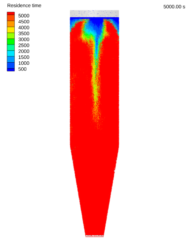
Figure 5: Residence time for cold-flow model
The model shows a distinct channel forming down the center of the vessel, which is consistent with observations reported in literature. Results show the residence time in a vertical cross-section of the vessel, showing lower residence time (more rapid downflow) in the center of the bed.
Reactive model
The results for the reactive model were compared with results from the REDUCTOR model reported in Hamadeh et al., 2018, showing a distinct central channel in the center in which solids reduction is slowed. For comparison with the REDUCTOR (2D) model, a similar Tecplot view was created in the center of the reactor using blanking constants. The variable shown here is the discrete particle mass fraction of each solids species.
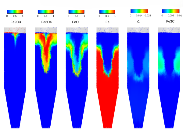
Figure 6: Discrete particle mass fractions at t = 2500s
For comparison, the equivalent view of the solids profiles is shown in the Hamadeh et al., 2018 paper in Figure 10. It should be noted that the REDUCTOR model does not account for hydrodynamics of the bed, as it is a 2D model. Therefore, reasonable differences in the distribution of solids can be expected.

Figure 7: Solids mass fractions from Hamadeh, 2018
Model results for the shaft furnace were compared with results from the 2D isometric model REDUCTOR as well as plant outlet gas compositions shown in the same paper (Hamadeh et al., 2018).
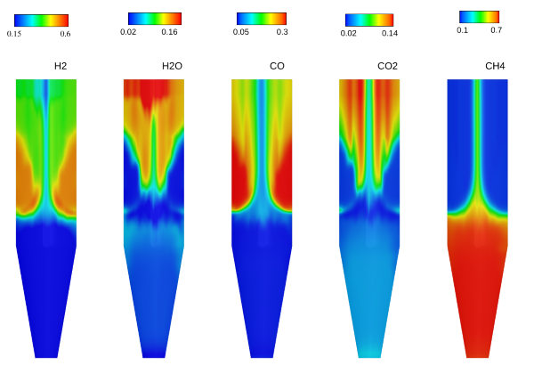
Figure 7: Gas species mole fractions at steady state (t = 2500s)
The model shows agreement with results from the 2D isometric model REDUCTOR cited in Hamadeh 2018. For reference, an image of the equivalent plots for this model is included below (Hamadeh et al., 2018).
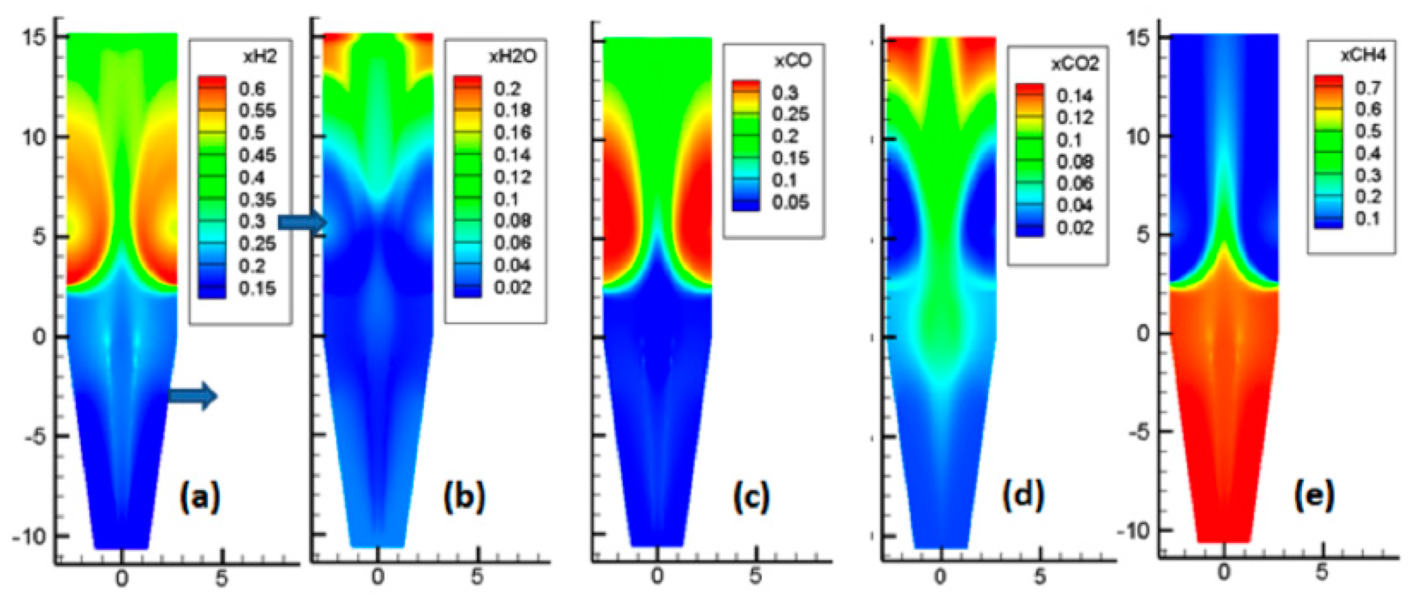
Figure 9: Gas species profiles from REDUCTOR model from Hamadeh et al. 2018
The general distribution of gases are similar between cases, with reducing agents hydrogen and carbon monoxide fed in through the reducing gas inlet and consumed as they travel up the moving bed. The model also shows the appearance of a central channel through the vessel in the reducing section, which is primarily composed of methane. This central channel is correlated with a lower rate of solids reduction and therefore provides a central channel for the unreduced solids to flow. Results for the composition of the outlet gases (averaged over the final 500 seconds of simulation run time) at the top of the furnace are compared with MIDREX plant operating data shown in Hamadeh 2018. The results show general agreement in the composition of the outlet gases:
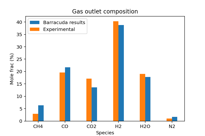
Figure 8: Gas outlet composition
Modeling Instructions
The user is expected to have already gone through basic Barracuda training: Barracuda Virtual Reactor New User Training | CPFD Software (cpfd-software.com).
- Download the support files provided along with this post. Due to the long runtime, an IC file is included in the project setup. The model is automatically restarted with the solids distribution close to steady state (at 2500s run time). If the user wishes to run with the original solids distribution, the model can be run by re-selecting all the Particle IC values and running the model from t = 0.
- Unzip the support file and place it in the working directory setup for this DRI shaft furnace project.
- Open a new Barracuda session.
- From the File menu, choose Open Project. Navigate to the working directory and select shaft_furnace.prj.
The project file has already been setup with the appropriate
- Grid
- Base Materials.
- Particles.
- Initial Conditions
- Fluid ICs.
- Particle Species.
- Boundary Conditions
- Pressure BCs.
- Flow BCs.
The chemistry setup for this project, which is already set up, is described below.
Chemistry
The reaction kinetics described in this post are input into Barracuda in the following manner:
- Solids reduction reactions are defined as discrete reactions. Gas-phase reactions are defined as stoichiometric reactions
- All rate constants are user-defined.
For the user-defined rate expressions for solids reduction, the general form of the UDE includes the following parameters:
- Kinv which refers to 1 + 1/Keq.
- Xi refers to the fraction of iron oxide species reduced, which is defined as the mass of the species being reduced divided by the total mass of the particle
- Ct refers to the molar concentration of gas
- CH2 refers to the molar concentration of Hydrogen
- CH2,eq refers to the molar concentration of Hydrogen at equilibrium (defined from Chaudron’s diagrams shown in Immonen and Powell, 2024)
The gas-phase reactions are also specified using user-defined chemistry. For both the water-gas shift and steam-methane reforming reaction, a separate forward and reverse reaction is specified. The following parameters are included based on the chemistry described in this post:
- Xi refers to the conversion of each iron oxide species
- F refers to the iron oxide reduction progress and is used to determine the value of the rate constant based on the value ranges specified.
- kn,i refers to the value of the rate constant, which depends on the value of the iron oxide reduction progress F using an IF statement
Time Controls
- Enter 0.01 seconds for the Time Step and 5000 secs for the End Time
- Put 500 seconds for the Restart Interval
Visualization Data
Ensure that the following Visualization Data outputs are selected in the Visualization Data tab in Figure 10.
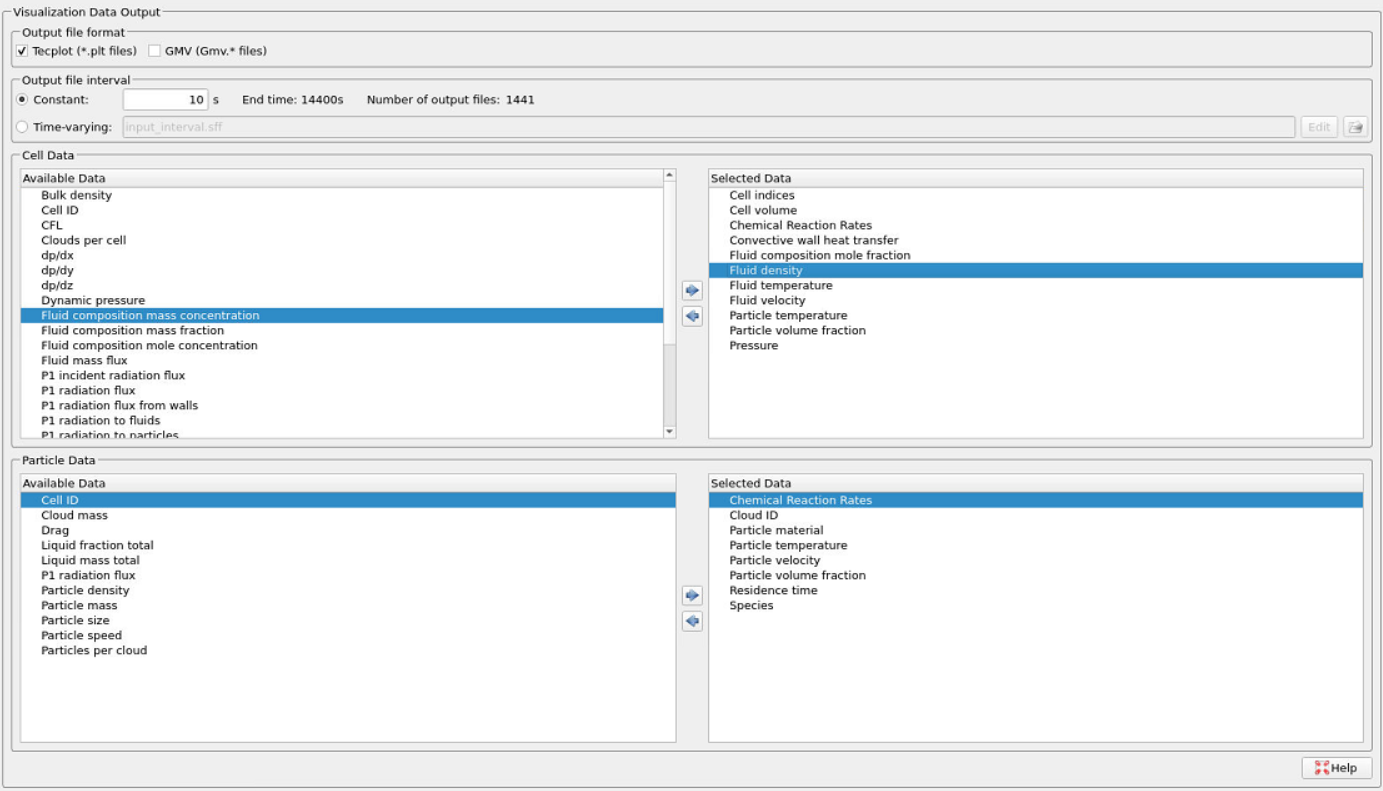
Figure 10: Visualization data output for MIDREX Shaft furnace simulation
Run
- Click on Run and then click on Run Solver
- Select GPU Parallel if you have the required GPU parallel license
Post Processing Shaft Furnace Results in Tecplot
The user is assumed to have gone through basic Tecplot training Getting Started With Tecplot For Barracuda® | CPFD Software (cpfd-software.com). So only a few brief steps for post processing the results are explained.
To create the contour plot shown in Figure 5, follow the steps shown below.
- In the Barracuda GUI click on Post-Run and then click on View Results.
- Deselect Scatter from the Plot menu.
- Select the checkbox next to Slices
- Select the gear icon next to Slices
- Under Definition, ensure that X-planes is selected from the Drop-down menu
- Under Contour tab, select the key icon to open the Contour and Multi-coloring details window
- Under the drop-down, select Fluid domain mole fraction H2(G)
- Under Color map options, select Modified Rainbow less green from the drop-down window.
- Select Continuous under Color map distribution method. Note that the min and max values under Contour values at endpoints will need to be manually updated based on the min and max values for the Contour legend
- Under the plot sidebar, select the ZY view from the list to get the appropriate view
- Select Frame -> Save frame style and save the frame style under a recognizable name such as H2_sliceView.sty
- Now that a single style-file has been generated, the frame style can now be used to create the equivalent view for other fluid species.
- Select the frame and press Ctrl + C to copy the frame. Create a copy of the same frame using Ctrl + V. Next, double click the contour bar and select Fluid domain mole fraction CO(G) to view the results for the CO mole fraction. Adjust min/max values in the Levels and Color tab as needed, ensuring that the bounds are also changed in the Color map distribution method window (below Color map)
- Once all relevant frames have been generated, select Frame -> Tile Frames and select the side-by-side view from the dropdown list to tile and organize the frames
To create the view of the solids profiles in Figure 8, follow the steps shown below:
- In the Barracuda GUI click on Post-Run and then click on View Results.
- Select Plot -> Blanking -> Value Blanking
- Select the Include value blanking checkbox. We want to blank out all regions of the domain except for a central thin slice to view the solids in the center
- Under Constraint 1, use the dropdown menu under Blank when to specify that 1:x should be blanked when it is less than or equal to -0.1. Ensure that the Active checkbox is selected
- Select Constraint 2 and use the dropdown options to specify that 1:x should be blanked when it is greater than or equal to 0.1. Ensure that the Active checkbox is selected. Select Close.
- Select ZY view from the Plot sidebar
- Double click on the geometry to open the Zone Style window. Navigate to the Scatter tab.
- On the zone titled Particles, which should be Group 1, right click on the highlighted Symbol shape. By default, it should be set to Point. From the list of options, select Sphere
- Right click on the Scatter size and select 1.0. This should increase the size of the particles significantly and render them as spheres
- Double click on the contour legend, and select Discrete particle mass fraction Fe2O3(S) from the dropdown menu
- Now that the spheres have been properly generated, select Frame -> Save frame style and choose a name for the frame such as Fe2O3_sliceView.sty. This can be used in the future to quickly generate the same frame view
- Copy and paste the frame in the manner shown in the previous section
- In the newly created frame, double click the contour legend and select Discrete particle mass fraction Fe3O4(S) from the dropdown list in the Contour and Multi-Coloring Details tab. This same view can be generated for all of the solids species.
- Once all relevant frames have been generated, select Frame -> Tile Frames and select the side-by-side view from the dropdown list to tile and organize the frames
References
Chipman, J. (1972). Thermodynamics and phase diagram of the Fe-C system. Metallurgical Transactions, 3(1), 55–64. https://doi.org/10.1007/bf02680585
Hamadeh, H., Mirgaux, O., & Patisson, F. (2018). Detailed modeling of the direct reduction of iron ore in a shaft furnace. Materials, 11(10), 1865. https://doi.org/10.3390/ma11101865
Immonen, J. (2023). GitHub – jimmonen11/DRI-furnace-model: DRI furnace model. GitHub. https://github.com/jimmonen11/DRI-furnace-model
Immonen, J., & Powell, K. M. (2024). Dynamic modeling of a direct reduced iron shaft furnace to enable pathways towards decarbonized steel production. Chemical Engineering Science, 300, 120637. https://doi.org/10.1016/j.ces.2024.120637
Meshram, A.; Korobeinikov, Y.; Nogare, D.D.; Zugliano, A.; Govro, J.; OMalley, R.J.; Sridhar, S. Modeling the First Hydrogen Direct Reduction Pilot Reactor for Ironmaking in the
USA Using Finite Element Analysis and Its Validation Using Pilot Plant Trial Data. Processes 2023, 11, 3346. https://doi.org/10.3390/pr11123346
Midrex Technologies, Inc. (2023). World Direct Reduction Statistics 2023.
Mondal, K., Lorethova, H., Hippo, E., Wiltowski, T., & Lalvani, S. (2004). Reduction of iron oxide in carbon monoxide atmosphere–reaction controlled kinetics. Fuel Processing Technology, 86(1), 33–47. https://doi.org/10.1016/j.fuproc.2003.12.009
Yu, S., Shao, L., Zou, Z., & Saxén, H. (2021). A Numerical Study on the Performance of the H2 Shaft Furnace with Dual-Row Top Gas Recycling. Processes, 9(12), 2134. https://doi.org/10.3390/pr9122134