
Introduction
For over a century, combustion technologies for energy production have been widely popular and effectively used. Dating back to advancements in steam engine technology made by Sir Charles Parsons of England in the late 1800s and Thomas Edison’s coal-fired power station in New York City, the concept of combustion-driven energy production has always existed in the modern industrial world. Traditionally, a coal feedstock is subjected to high temperatures to generate steam, which drives a turbine or an equivalent prime mover, then generating energy in the form of electricity. There is a clear transition of thermal energy generated from combustion to mechanical energy to electrical energy that drives and enables the modern world. In the last forty years, a significant adoption made by companies looking to implement improved combustion processes is the usage of circulating fluidized bed (CFB) technology.
The boiler is the beating heart of traditional power plants, and advancements in boiler technology have manifested in the CFB combustor, greatly improving the overall process. CFBs can be divided into several sections, as seen in Figure 1. Zone 1 is commonly referred to as the riser, where gas-solid interactions are to take place, eventually leading to combustion and heat generation. Air is fed through a primary air inlet (zone 3) and contacted with solid fuel particles being fed from a hopper (zone 2). This section of the riser is known as the dense zone and is typically packed with solids and intensely fluidized as if it were a boiling liquid. In this zone, particles collide frequently, providing excellent mixing of fuels and air, promoting complete and efficient combustion. Secondary air is fed from zone 4 and leads into the transition zone, in which the fluidization characteristics become less intense, caused by a higher gas velocity. There begins to exist a particle size gradient with smaller particles being entrained upwards with the fluidizing medium. Above this secondary air inlet in the riser portion exists the dilute zone in which particles are carried to a cyclone separator in zone 5. The dilute zone is mainly dominated by gas-solid interactions, and following the cyclone, gases are returned to the system in zone 6 via a loop seal.
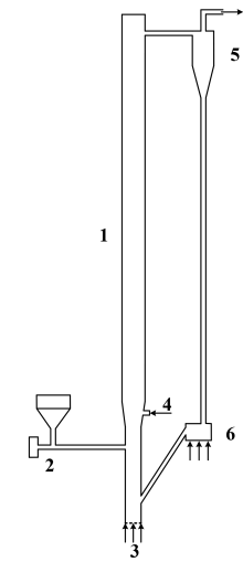
Figure 1: Circulating Fluidized Bed

Figure 2: Power plant with CFB Combustor
Functionally, the CFB combustor operates by fluidizing a bed of particles using air through the primary air inlet. The bed of particles consists of solid fuel (coal, biomass, waste, etc), char from combusted solids, ash, added inert substances like sand, and added sorbents like limestone. The volatile species held within the fuel will be released and reacted upon interacting with fluidizing air. These volatile species will begin a series of reactions, many of which are exothermic, generating a significant amount of heat. These reactions occur throughout the riser section of the CFB, and the heat generated will be utilized in the power plant’s operation. The particles will then be carried through the outlet of the riser and into a cyclone, where they will be separated and returned to the riser at a lower section and a higher average temperature, thus creating the “circulating” nature of the process. There are several reasons why CFB combustors are widely accepted as an improvement in combustion technology. CFB combustors are incredibly fuel flexible, meaning they can accept a wide variety of fuel types of differing qualities. Biomass, waste materials, natural gas, and even low-grade coals can be used as feedstock, allowing for diversification of fuel sources and a decrease in operational cost. CFB combustors also produce less NOx and SOx due to a lower average combustion temperature when compared to a traditional boiler, and the usage of sorbents like limestone to absorb sulfur oxides. Overall, harmful emissions are therefore lowered, and the need for external flue gas treatment downstream of the CFB is eliminated. The nature of particles circulating through the riser mixing with the fuel and released volatiles allows for very efficient heat transfer and a large heat transfer surface area, leading to greater combustion efficiency and less waste of feedstock. In essence, CFB combustors are efficient, more environmentally friendly than their predecessors, and cost-efficient. After the CFB combustor in an overall power plant process (Figure 2), hot flue gas from the cyclone separator is passed through a heat exchanger in which water is flown. The heat produced from combustion in the CFB provides enough energy to vaporize water to steam, which is then compressed and used to move a prime mover such as a turbine or screw. This mechanical movement is then converted to electrical energy that can be supplied to infrastructure across the globe.
For this application model, several aspects of the CFB were omitted, and assumptions were made to account for their omission. Only the riser portion of the CFB is modeled in this simulation with an appropriate primary, secondary, coal, and recycle inlet. All model parameters and specifications were taken from the work of Wu et al’ 2017 and their work with a physical 50 kW CFB combustor.
Model Definition
This application model exemplifies the usage of a compressible domain with volumetric reaction chemistry in Barracuda Virtual Reactor (Barracuda). The CFB geometry stems from a physical CFB described in the work of Wu et. al’ 2017. As mentioned previously, the riser portion of the CFB is the focus of the model, as seen in Figure 3, which displays the model geometry in Barracuda. The riser is 4.2 meters (m) tall with three zones: A dense zone (0 – 0.8 m), a transition zone (0.8 – 1 m), and a dilute zone (1 – 4.2 m). The inner diameter of the riser up until the transition zone is 0.122 m, and the dilute zone experiences an increase in inner diameter to 0.15 m. The riser walls for the dense and transition zones are treated as adiabatic walls. The wall temperature in the dilute zone is fixed at 298 K, and a thermal wall resistance is specified to capture heat loss. The domain is initialized (between 0 and 0.4 m) with a bed of ash and CaO particles. The particle species used in this experiment are bituminous coal feed (contains volatiles as well) and devolatilized coal, which is composed primarily of ash and some CaO. The composition of coal particles is determined from the proximate and ultimate analysis of the coal type provided in Wu 2017. The enthalpy of devolatilization is obtained from the heating value provided in Wu 2017. Both particle species are set to a uniform particle diameter of 0.35 mm. The Radl-Sundaresan drag model is used to capture the fluid-solid drag interaction for both particle species. From Wu et al’ 2017, a coal mass flow rate is specified at 0.00212 kg/s. Using the specified practical gas flow (m3 /kg coal) and the air density, the total mass of air per kg of coal was calculated and multiplied by the coal mass flow rate to determine the total flow rate of air in the system. Ratios for primary air, secondary air, material returning air, and coal distributing air were each specified from the paper and multiplied with the total air flow to determine mass flow through each inlet (Primary air: 0.0112 kg/s, Secondary air: 0.0056 kg/s, recycle air: 0.0009 kg/s, coal distributing air: 0.0009 kg/s) with air being defined as 21% molecular oxygen and 79% molecular nitrogen. Flow BC’s are specified for each of the inlets, and a BC connector is used to return all particles from the outlet pressure BC to the recycle inlet (it is assumed that the cyclone is 100% efficient). A pressure drop of 50 Pa is specified at the outlet, and the inlets are all assumed to operate at atmospheric pressure. Finally, all base compounds and materials specified are functions of temperature, and all fluids are assumed to be ideal in nature.
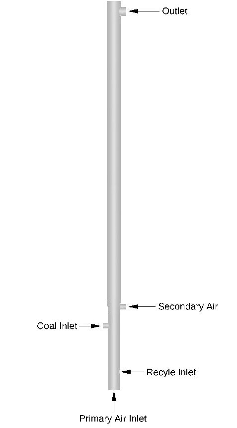
Figure 3: CFB Riser Geometry
Reaction Kinetics
The kinetic model for the CFB combustion process came from several sources, with reactions 1-4, 6-7, 9-12, 14, 16, and 18-19 coming from Krusch 2018. Additionally, reactions 5 and 15 are taken from Wu, 2017; reactions 13, 24, and 25 stem from Xie, 2017; reaction 17 and the discrete reaction for CaO absorption of SO2 come from Xie, 2014. A complete list of sources is provided further below, and a full reaction set is available through the provided support file. The reaction set consists of fluid phase volumetric reactions as well as discrete reactions in which volatile species are released. Two reactions are also to be user-defined and are specified in this instruction set. The source of reactants in the overall system stems from the release of volatiles (CO, CO2, CH4, Soot, H2, H2S, HCN, and NH3) held within the coal particles. The first set of reactions in the kinetic model occurs in the gas phase and covers the main set of reactions for hydrocarbons in the system (reactions 0-8). A set of reactions was also included to accurately model reactions of nitrogen species (9-12, 14, 16-17, 24-25, 27), and a reaction for the formation of sulfur dioxide can be seen in reaction 20. Several char surface reactions are also included in this model in which carbon on the coal particle’s surface reacts with the volatile species and those formed from reactions (13, 15, 18-19, 26). The reaction set is shown in detail below.
$$ CO + H_2O \rightarrow CO_2 + H_2 \quad \text{(1)} $$
$$ CO_2 + H_2 \rightarrow CO + H_2O \quad \text{(2)} $$
$$ CH_4 + 1.5O_2 \rightarrow CO_2 + 2H_2O \quad \text{(3)} $$
$$ 2H_2 + O_2 \rightarrow H_2O \quad \text{(4)} $$
$$ CO + 0.5O_2 \rightarrow CO_2 \quad \text{(5)} $$
$$ C(s) + H_2O(v) \rightarrow CO + H_2 \quad \text{(6)} $$
$$ C(s) + CO_2 \rightarrow 2CO \quad \text{(7)} $$
$$ Soot + O_2 \rightarrow CO_2 \quad \text{(8)} $$
$$ HCN + 1.25O_2 \rightarrow NO + CO + 0.5H_2O(v) \quad \text{(9)} $$
$$ HCN + NO + 0.75O_2 \rightarrow N_2O + CO + 0.5H_2O(v) \quad \text{(10)} $$
$$ NH_3 + NO + 0.25O_2 \rightarrow N_2 + 1.5H_2O(v) \quad \text{(11)} $$
$$ NO + CO \rightarrow 0.5N_2 + CO_2 \quad \text{(12)} $$
$$ NO + C(s) \rightarrow 0.5N_2 + CO \quad \text{(13)} $$
$$ NH_3 + 1.25O_2 \rightarrow NO + 1.5H_2O(v) \quad \text{(14)} $$
$$ N_2O + C(s) \rightarrow N_2 + CO \quad \text{(15)} $$
$$ NH_3 + 0.75O_2 \rightarrow 0.5N_2 + 1.5H_2O(v) \quad \text{(16)} $$
$$ H_2S + 1.5O_2 \rightarrow SO_2 + H_2O(v) \quad \text{(17)} $$
$$ C(s) + 0.5O_2 \rightarrow CO \quad \text{(18)} $$
$$ C(s) + O_2 \rightarrow CO_2 \quad \text{(19)} $$
$$ S(s) + O_2 \rightarrow SO_2 \quad \text{(20)} $$
$$ N(s) + 0.5O_2 \rightarrow NO_2 \quad \text{(21)} $$
$$ H(s) + 0.25O_2 \rightarrow 0.5H_2O(v) \quad \text{(22)} $$
$$ O(s) \rightarrow 0.5O_2 \quad \text{(23)} $$
$$ N_2O + CO \rightarrow N_2 + CO_2 \quad \text{(24)} $$
$$ N_2O \rightarrow N_2 + 0.5O_2 \quad \text{(25)} $$
$$ NO + 0.5C(s) \rightarrow 0.5N_2 + 0.5CO_2 \quad \text{(26)} $$
$$ N_2 + O_2 \rightarrow 2NO \quad \text{(27)} $$
The rate law for each respective reaction is also shown below. Two additional discrete reactions are also included in the reaction set that will be discussed and defined later in this post.
\begin{align}
R_0 &= k_0 [CO]^{0.5} [H_2O(v)] \\
R_1 &= k_1 [H_2]^{0.5} [CO_2] \\
R_2 &= k_2 [CH_4]^{-0.3} [O_2]^{1.3} \\
R_3 &= k_3 [H_2]^{0.5} [O_2] \\
R_4 &= k_4 [CO] [H_2O(v)]^{0.5} [O_2]^{0.5} \\
R_5 &= \left(k_6 [H_2O(v)] \right) – \left(k_7 [H_2] [CO] \right) \\
R_6 &= \left(k_8 [CO_2] \right) – \left( k_9 [CO]^{2} \right) \\
R_7 &= k_{26} [Soot] [O_2]^{0.5} \\
R_8 &= \frac{\left( k_{18} [HCN] [O_2] \right)} { \left( 1+ k_{19} [NO] \right)} \\
R_9 &= \frac{\left(k_{19} [NO] \right) \left(k_{18} [HCN] [O_2] \right) } {\left(1 + k_{19} [NO] \right)} \\
R_{10} &= k_{10} [NH_3]^{0.5} [NO]^{0.5} [O_2]^{0.5} \\
R_{11} &= \frac{\left( k_{21} \left(186.2[NO] \right)\right) \left(7.86[CO] + 0.002531 \right)} {186.2[NO] + 7.86[CO] + 0.002531} \\
R_{12} &= k_{35} [NO] \\
R_{13} &= k_{23} [NH_3][O_2] \\
R_{14} &= k_{35} [N_2O] \\
R_{15} &= k_{31} [NH_3] [O_2] \\
R_{16} &= k_{29} [H_2S] [O_2] \\
R_{17} &= \frac{k_{13} [O_2]} {1 + k_{12}} \\
R_{18} &= \frac{k_{13} [O_2] k_{12} } {1 + k_{12}} \\
R_{19} &= k_{14} [O_2] \\
R_{20} &= k_{15} [O_2] \\
R_{21} &= k_{16} [O_2] \\
R_{22} &= k_{17} [O_2] \\
R_{23} &= k_{32} [N_2O] [CO] \\
R_{24} &= k_{33} [N_2O] \\
R_{25} &= k_{35} [NO] \\
R_{26} &= k_{36} [N_2] [O_2]^{0.5}
\end{align}
The rate constants for the above reactions are given below, as they need to be input in Barracuda. All conversions and modifications have been made and explained in detail under the Modeling Instructions section of this post. Constants k12 and k28 are omitted from this portion and will be specified further in the post.
\begin{align}
k_0 &= 7.7 \times 10^{10} \exp\left(\frac{-36640}{T} \right) \\
k_1 &= 6.4 \times 10^{9} \exp\left(\frac{-39200}{T} \right) \\
k_2 &= 1.5 \times 10^{7} \exp\left(\frac{-15098}{T} \right) \\
k_3 &= 1.6 \times 10^{9} \exp\left(\frac{-10000}{T} \right) \\
k_4 &= 1.3 \times 10^{11} \exp\left(\frac{-15100}{T} \right) \\
k_5 &= 2.7 \times 10^{8} \exp\left(\frac{-20131}{T} \right) \\
k_6 &= 6.4T \theta_{f} \exp\left(\frac{-22645}{T} \right) m_{C} \\
k_7 &= 0.0005218 T^{2} \theta_{f} =\exp\left(\frac{-6319}{T – 17.29} \right) m_{C} \\
k_8 &= 6.4 T \theta_{f} \exp\left(\frac{-22645}{T} \right) m_{C} \\
k_9 &= 0.0005218 T^{2} \theta_{f} \exp\left(\frac{-6319}{T -17.29} \right) m_{C} \\
k_{10} &= 214000 \exp\left(\frac{-10000}{T} \right) \\
k_{11} &= 1.02 \times 10^{9} \exp\left(\frac{-25460}{T} \right) \\
k_{13} &= 859 \exp\left(\frac{-18000}{T} \right) A_{C} \\
k_{14} &= 322 \exp\left(\frac{-18000}{T} \right) A_{S} \\
k_{15} &= 736 \exp\left(\frac{-18000}{T} \right) A_{N} \\
k_{16} &= 103100 \exp\left(\frac{-18000}{T} \right) A_{H} \\
k_{17} &= 644 \exp\left(\frac{-18000}{T} \right) A_{O} \\
k_{18} &= 214000 \exp\left(\frac{-10000}{T} \right) \\
k_{19} &= 1.02 \times 10^{9} \exp\left(\frac{-25460}{T} \right) \\
k_{20} &= 3.4785 \times 10^{13} \exp\left(\frac{-27676}{T} \right) \\
k_{21} &= 1.952 \times 10^{7} \exp\left(\frac{-19004}{T} \right) \\
k_{22} &= 5.85 \times 10^{7} \exp\left(\frac{-12000}{T} \right) A_{C} \\
k_{23} &= 3.1 \times 10^{8} \exp\left(\frac{-10000}{T} \right) \\
k_{24} &= 2.9 \times 10^{9} \exp\left(\frac{-16983}{T} \right) A_{C} \\
k_{25} &= 5.017 \times 10^{14} \exp\left(\frac{-35200}{T} \right) \\
k_{26} &= 3.9 \times 10^{6} \exp\left(\frac{-16959}{T} \right) \\
k_{29} &= 5.2 \times 10^{8} \exp\left(\frac{-2.32}{T} \right) \\
k_{30} &= 11400 \exp\left(\frac{-8780}{T} \right) m_{Volatile} \\
k_{31} &= 4.96 \times 10^{8} \exp\left(\frac{-10000}{T} \right) \\
k_{32} &= 1.24 \times 10^{9} \exp\left(\frac{-5913.3}{T} \right) \\
k_{33} &= 1.5 \times 10^{11} \exp\left(\frac{-20159}{T} \right) \\
k_{34} &= 130000 \exp\left(\frac{-1711}{T} \right) \\
k_{35} &= 6 \times 10^{-10} \theta_{f} d_{all} {vf}_{C}^{0.333} {vf}_{all}^{0.667} \\
k_{36} &= 2.6358 \times 10^{10} T^{-0.5} p^{0.5} \exp\left(\frac{-51934.3}{T} \right)
\end{align}
Results and Discussion
Figure 4 shows the initial fluidization of devolatilized coal (ash + CaO) in the riser as well as the particle dynamics of coal particles in the system. A bed of devolatilized coal particles is initialized in the first 0.4 meters of the riser, forming a turbulently circulating bed along with coal quickly after air is introduced to the system. Figure 4a displays the fluidization behavior for 60 seconds, showing the circulation of particles throughout the system. The traveling of devolatilized coal throughout the bed is key to achieving efficient heat transfer, as it serves as the primary vessel for heat as reactions occur and heat is evolved. As the coal particles circulate through the CFB, carbon present at the particle’s surface will react in a series of char reactions. Figure 4b displays the mass fraction of carbon present in each coal particle, and as time evolves, more and more particles with no carbon are seen entrained in the flow of air. The surface char reactions produce compounds like CO, HCN, and CO2, and the gradual decline of carbon in coal particles is evidence of such reactions happening in the system. Volatile species are also released from the introduced coal particles quickly, and Figure 4c displays the rapid devolatilization of fresh coal feed as the particles are fed into fluidizing air. Coal particles seem to release all volatiles almost instantaneously, reflected by a sharp drop in volatile mass fractions on the feed particles from 24 to 0%. An additional layer of emissions control within the CFB is the inclusion of CaO, a sorbent that reacts with SO2, forming solid CaSO4. Figure 4d depicts the predicted mass fraction of CaSO4 deposited on the devolatilized coal. Over time, the particles adsorb surrounding CO2 and become loaded at a mass fraction of 0.0018.
Figure 5 shows the Barracuda simulation predicted O2, CO2, SO2, and NO mole fractions as well as the riser’s varying fluid temperature over 60 seconds. Figure 5a depicts O2 gas distribution across the riser. In the fuel-dense zone at the bottom of the CFB, air is fed and consumed quickly by volatile species and eventually recycled coal, forming hydrocarbon compounds and CO/NO. Moving up the riser, we see a sharp decrease in O2 above the height of the secondary air inlet. Fresh oxygen from this zone re-oxidizes any NO and CO that have not been further reduced to form NOx and CO2. Figure 5b shows that the CO2 distribution reflects this, as high CO2 concentrations only exist above the primary air inlet, essentially after CO from the dense zone has been oxidized along with CO2 produced via char reaction. Fresh secondary air also oxidizes NO that has not been reduced to molecular nitrogen, thus promoting the formation of NOx compounds. In Figure 5c showing NOx formation, there is a clear increase in NO production right above the secondary inlet, reflecting this notion. Experimental results from a physical model of this same CFB combustor are compared with the Barracuda simulation results in Figures 6 and 7. Figure 6 shows a comparison of the time-averaged outlet gas volume fraction of O2 and CO2 between the simulated and experimental results, showing a good match. The Barracuda predicted O2 and CO2 mole fractions on a dry basis are 3.22% and 14.625% respectively. Figure 7 shows the average fluid temperature along the height of the riser. Again, a good match is observed between the simulation and experimental results. The production of NOx and SO2 in the simulation was approximately 713 and 118 ppm, respectively. Minor discrepancies between the experimental and Barracuda simulation results can be associated with significant differences in the kinetic models used for both.
Figure 4a: Circulation of fresh coal feed and devolatilized coal through the riser. 4b: Mass fraction of carbon in coal particles over time. 4c: Mass fraction of volatiles present in coal particles. 4d: Mass fraction of CaSO4 in devolatilized coal.
Figure 5a: Mole fraction distribution of O2. 5b: Mole fraction distribution of CO2. 5c: Mole fraction distribution of NO. 5d: Mole fraction distribution of SO2. 5e: Fluid temperature through the riser.
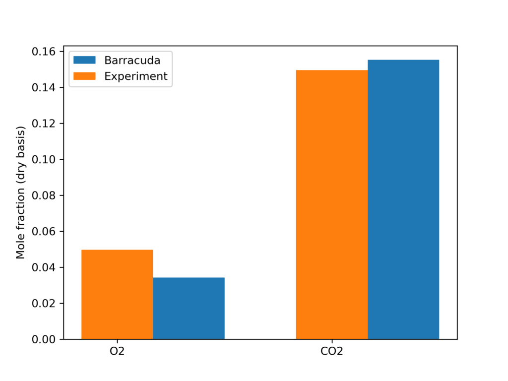
Figure 6: Outlet O2 and CO2 composition comparison between the experiment and Barracuda simulation
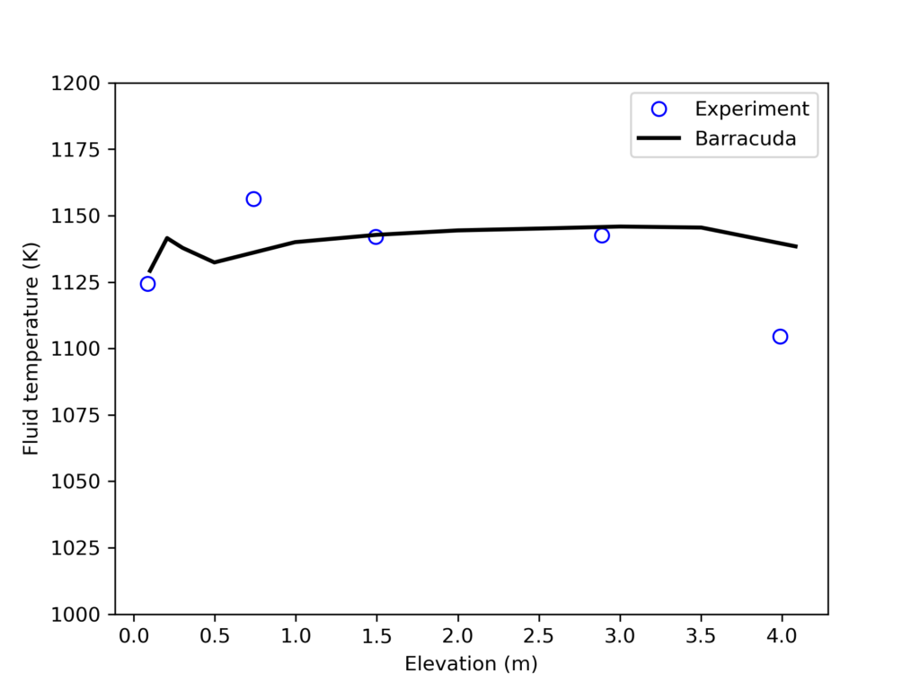
Figure 7: Fluid Temperature Comparison Between Barracuda Simulation and Experiment.
Modeling Instructions
Circulating Fluidized Bed (CFB) Combustor Simulation Setup
The user is expected to have already gone through basic Barracuda training, Barracuda Virtual Reactor New User Training | CPFD Software (cpfd-software.com).
- Download the support files provided along with this post.
- Unzip the support file and place it in the working directory set up for this CFB project.
- Open a new Barracuda session.
- From the File menu, choose Open Project. Navigate to the working directory and select CFB.prj.
The project file has already been set up with the appropriate
- Grid.
- Base Materials.
- Particles.
- Initial Conditions
- Fluid ICs.
- Particle Species.
- Boundary Conditions
- Pressure BCs.
- Flow BCs.
- Chemistry
The chemistry setup for this project, which is already complete, is described in detail below.
Chemistry
Rate Coefficients
Many of the rate coefficients seen in the kinetic model (such as k0) follow the standard Arrhenius form, only requiring a pre-exponential factor (C0) and an activation energy to be specified. Several rate constants include a particle dependence specification resulting in the overall rate being influenced by the total mass (k6), volume fraction (k35), diameter (k35), or area (k13) of a specific species. A common inclusion in the kinetics is a term that accounts for the volume of fluid present in a given control volume (θf). The instructions below describe the setup of the rate constant k9, which encompasses all of the previously described parameters.
- Under Chemistry, select Rate Coefficients. Click Add to bring up the Chemistry Coefficient Editor. Volume-Average, which is the default reaction type, is used for this rate constant.
- Add the following equation parameters shown in Figure 7.
- Enter a value of 0.0005218 for C0, the pre-exponential factor.
- Enter a value of 2 for C1 to account for the second-order temperature value (T2).
- Enter a value of 1 for C4 to account for the volume of fluid present θf.
- Specify an activation energy of 6319 and an initial activation energy of -17.29.
- Select Particle Dependence in the Chemistry Coefficient Editor
- From the Project Materials List, add C to the Materials List, selecting mass for the Material Coefficient Type.
- Select a mass unit of kg/m3.
Entering the rest of the rate constants follows a similar procedure, ensuring that the correct particle dependences and parameters are accounted for in each respective equation. All of the rate constant equations are intended for volume average chemistry, apart from k30 and k28, which are to be used for discrete rate expressions. The discrete reactions must be specified differently and are for heterogeneous reactions occurring directly on the surface of the particles, with volume average chemistry being concerned with homogeneous reactions. Two of the rate constant expressions are user-defined (k12 and k28), and their expressions are shown below in Figures 5 and 6.
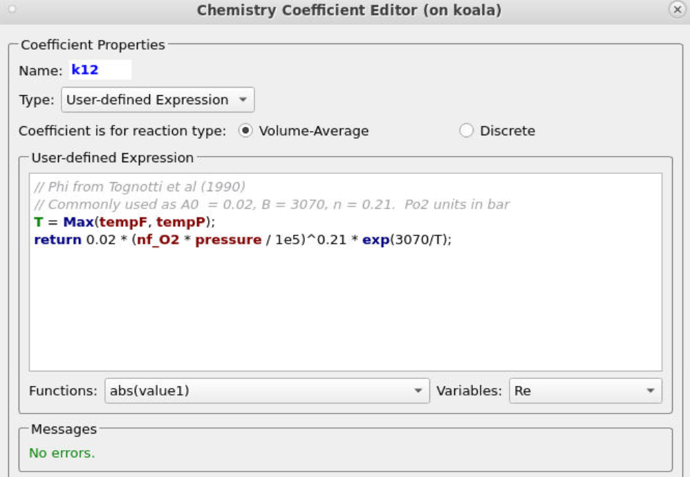
Figure 5: User-Defined Expression for k12
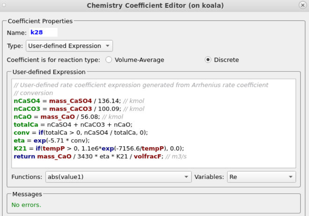
Figure 6: User-Defined Expression for k28
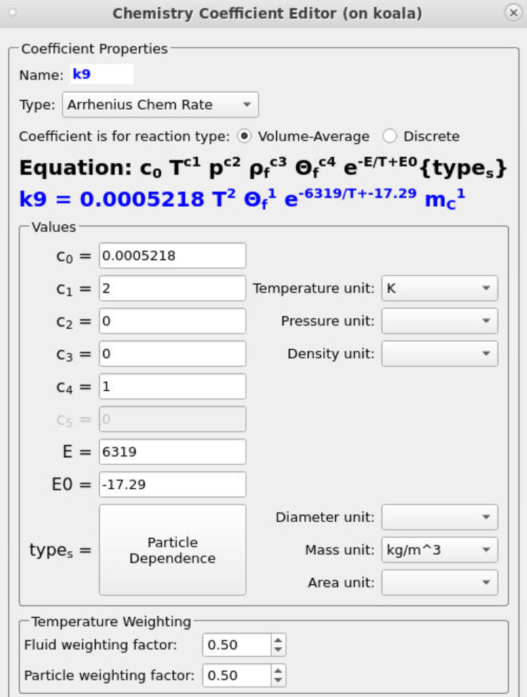
Figure 7: Arrhenius Expression for k9
Reactions
The reaction set included in this kinetic model comprises 29 reactions. 27 of these reactions occur in the fluid phase and follow homogeneous volume average chemistry. The procedure for entering reactions in Barracuda is shown below using reaction 1 and rate expression 0 as an example.
- Under Chemistry, select Reactions. Click Add ⇒ Volume-Average: Stochiometric rate equation to bring up the Chemistry Stochiometric Equation Editor.
- Under Equations Units, select mol/m3/sec for Reaction rate units and mol/m3 for Fluid species units.
- Enter the Stoichiometric reaction for water gas shift as shown in Figure 8.
- Enter the rate equation R0 for the stoichiometric reaction as shown in the box R00.
- Click OK to close the Chemistry Stochiometric Equation Editor.
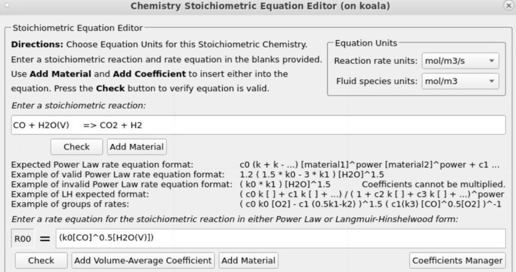
Figure 8: Water Gas Shift Reaction Stoichiometry
The two discrete reactions must be specified in another manner. The first discrete reaction is shown in Figure 9 and specifies the rates at which volatile species are to be released from the coal fed into the system. The rate is based on the mass of volatiles being released per unit time, and it is specified as kg/s. The rates at which each species is released are calculated with knowledge of the coal species composition and are crucial in determining an accurate composition throughout the system. The CaO contained in the ash can absorb a part of SO2 into calcium sulfate, CaSO4; this discrete reaction setup is shown in Figure 10.
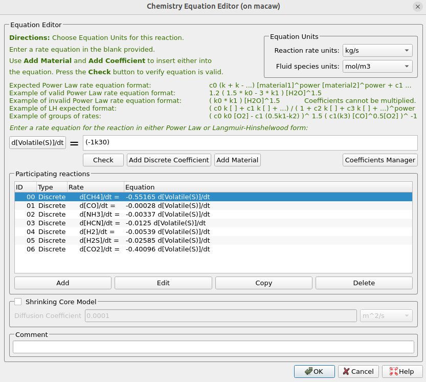
Figure 9: Volatile Release
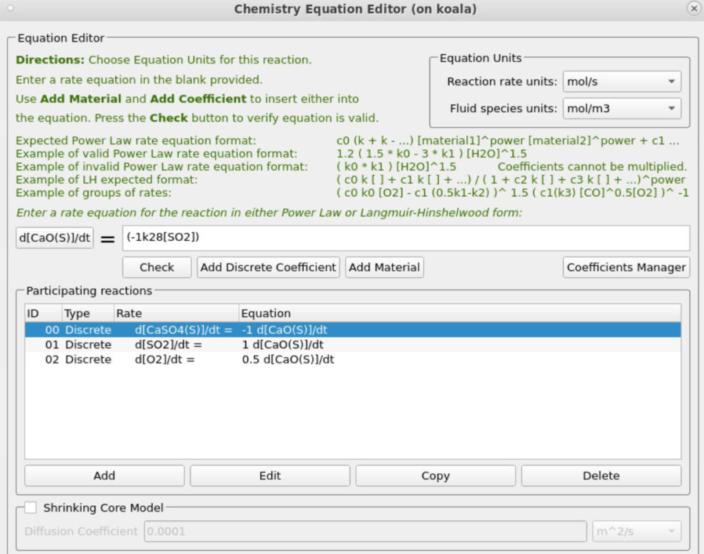
Figure 10: SO2 Release
Time Controls
- Enter 1.5e-4 secs for Time Step and 60 secs for End Time.
- Put 0.1 secs for the Restart Interval.
Visualization Data
- Enter 0.2 secs for the Output file interval.
- Select the Visualization Data for post-processing as shown in Figure 11.
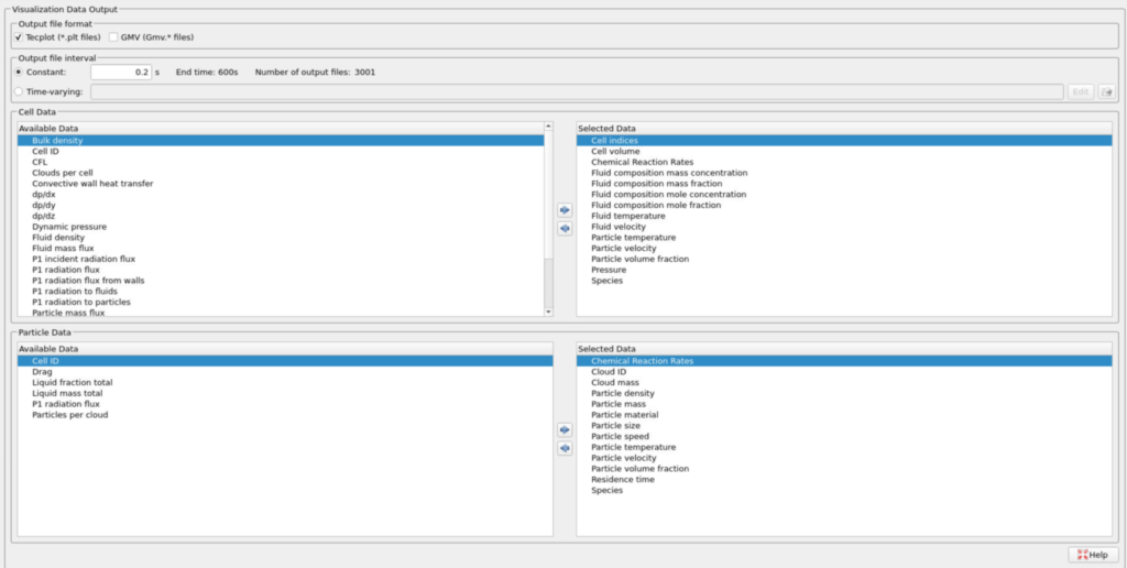
Figure 11: Selected Visualization Data for CFB Combustor Model
Run
- Click on Run and then click on Run Solver.
- Select GPU Parallel if you have the required GPU parallel license.
Post-Processing CFB Combustor Results in Tecplot
The user is assumed to have gone through basic Tecplot training, Getting Started With Tecplot For Barracuda® | CPFD Software (cpfd-software.com), and the training material in “Tecplot for Barracuda – Using frames” (Tecplot for Barracuda – Using Frames | CPFD Software (cpfd-software.com)). Only a few brief steps for post-processing the results are explained.
The following set of instructions is intended for the reproduction of the animations in Figure 4.
- In the Barracuda GUI, click on Post-Run and then click on View Results.
- Navigate to File, Load Barracuda Data, and select to Refresh / Reload All from the dropdown menu.
- Copy the entire frame and paste it three times, then tile the frames by selecting Frame, Tile Frames, and selecting the vertical option.
- Select Frame, Frame Linking, check the Solution Time option, and Apply Settings to all Frames in this Group.
- The following instructions are for Figure 4a:
- Snap the orientation view to ZX and zoom accordingly.
- From the Quick Macro bar, select Particles/Bubbles: Species.
- Double click on the contour bar, navigate to Levels and Colors, and Set Levels from 2 to 3 with 2 steps.
- Under Levels and Colors, set the color map to Diverging Blue/Yellow/Red.
- The following instructions are for Figure 4b:
- Snap the orientation view to ZX and zoom in, focusing on the coal inlet and the riser section above it.
- Double-click the contour bar and under variable select Discrete particle mass fraction C(S).
- Navigate to Plot, Blanking, Value Blanking, and blank when the species is not equal to 2.
- Navigate to Levels and Colors in the contour options and Set Levels to 0 to 0.6 using 6 steps.
- Also in Levels and Colors, select the continuous option and set the min and max to 0 and 0.6.
- Select Zone Style, navigate to the Scatter tab, and change the Particle Symbol Shape to Spheres.
- In the same tab, right-click on Scatter Size, select Select Variable, choose Particle Size, and select Close.
- Navigate again to the Particle Size tab, this time selecting the Particle Size variable option that is now available.
- Again, navigating to the Particle Size dropdown, select the Select Variable option, input a value of 2.55e-05 for the Grid units/magnitude, and select Close.
- Under Zone Style, Shade, set the cell color to white.
- Navigate to Zone Style, Effects, and set the Cells Surface Translucency to 80%.
- Navigate to Legend in the contour options and uncheck the Separate color bands option.
- Also under Legend, change the Header text to Use Text and title the contour mF Carbon.
- The Following instructions are for Figure 4c:
- Snap the orientation zoom to ZX and zoom in on the coal inlet.
- Double click the contour bar and under variable select Discrete particle mass fraction Volatile(S).
- Navigate to Plot, Blanking, Value Blanking, and blank when the species is not equal to 2.
- Navigate to Levels and Colors in the contour options and Set Levels to 0 to 0.24 using 5 steps.
- In Levels and Color, set the color map to Doppler.
- Also in Levels and Colors, select the continuous option and set the min and max to 0 and 0.24.
- Select Zone Style, navigate to the Scatter tab, and change the Particle Symbol Shape to Spheres.
- In the same tab, right-click on Scatter Size, select Select Variable, choose Particle Size, and select Close.
- Navigate again to the Particle Size tab, this time selecting the Particle Size variable option that is now available.
- Again, navigating to the Particle Size dropdown, select the Select Variable option, input a value of 1.5e-05 for the Grid units/magnitude, and select Close.
- Under Zone Style, Shade, set the cell color to white.
- Navigate to Zone Style, Effects, and set the Cells Surface Translucency to 80%.
- Navigate to Legend in the contour options and uncheck the Separate color bands option.
- Also under Legend, change the Header text to Use Text and title the contour mF Volatiles.
- The following instructions are for Figure 4d:
- Snap the orientation zoom to ZX and fit the entire domain accordingly.
- Double click on the contour bar, navigate to Levels and Colors, and change the variable to Discrete Particle Mass Fraction CaSO4(S).
- In Levels and Colors, change the color map to Modified Rainbow Dark Ends, setting the levels to 0 and 0.0018 with 3 steps.
- Select the continuous color map option, setting a min and max of 0 and 0.0018.
- Under Legend, uncheck the Separate Color Bands option.
- Also under Legend, change the Header text to Use Text and title the contour mF CaSO4.
The following set of instructions pertains to the recreation of Figure 5 animations.
- In the Barracuda GUI, click on Post-Run and then click on View Results.
- Navigate to File, Load Barracuda Data, and select to Refresh / Reload All from the dropdown menu.
- Copy the entire frame and paste it four times, then tile the frames by selecting Frame, Tile Frames, and selecting the vertical option.
- Select Frame, Frame Linking, check the Solution time and 3d plot view options, and Apply Settings to all Frames of this Group.
- The set of instructions below is intended to reproduce Figure 5a:
- Snap the orientation zoom to ZX and fit the entire domain accordingly.
- From the Quick macros options, select Cells: Fluid Temperature.
- Double-click on the contour bar and change the variable to Fluid domain mole fraction O2(g).
- Under Levels and Colors, Set Levels to 0 to 0.2 using 5 steps, and change the color map option to Sequential – Blue.
- Select the continuous color map distribution option, setting the min and max to 0 and 0.2.
- Under Legend, uncheck the separate color bands option, and position the legend at X:3.75, Y:99.1.
- Under Legend, change the Header text to Use Text and set the header to nF O2.
- The set of instructions below is intended to reproduce Figure 5b:
- Snap the orientation zoom to ZX and fit the entire domain accordingly.
- From the Quick macros options, select Cells: Fluid Temperature.
- Double-click on the contour bar and change the variable to Fluid domain mole fraction CO2(g).
- Under Levels and Colors, Set Levels to 0 to 0.19 using 5 steps, and change the color map option to Sequential – Orange.
- Select the continuous color map distribution option, setting the min and max to 0 and 0.19.
- Under Legend, uncheck the separate color bands option, and position the legend at X:3.75, Y:99.1.
- Under Legend, change the Header text to Use Text and set the header to nF CO2.
- The set of instructions below is intended to reproduce Figure 5c:
- Snap the orientation zoom to ZX and fit the entire domain accordingly.
- From the Quick macros options, select Cells: Fluid Temperature.
- Double-click on the contour bar and change the variable to Fluid domain mole fraction NO(g).
- Under Levels and Colors, Set Levels to 0 to 0.0016 using 5 steps, and change the color map option to Sequential – Purple/Red.
- Select the continuous color map distribution option, setting the min and max to 0 and 0.0016.
- Under Legend, uncheck the separate color bands option, and position the legend at X:3.75, Y:99.1.
- Under Legend, change the Header text to Use Text and set the header to nF NO.
- The set of instructions below is intended to reproduce Figure 5d:
-
- Snap the orientation zoom to ZX and fit the entire domain accordingly.
- From the Quick macros options, select Cells: Fluid Temperature.
- Double-click on the contour bar and change the variable to Fluid domain mole fraction SO2(g).
- Under Levels and Colors, Set Levels to 0 to 0.01 using 5 steps, and change the color map option to Sequential – Green/Blue, ensuring to check the reverse color map option.
- Select the continuous color map distribution option, setting the min and max to 0 and 0.01.
- Under Legend, uncheck the separate color bands option, and position the legend at X:3.75, Y:99.1.
- Under Legend, change the Header text to Use Text and set the header to nF SO2.
-
- The set of instructions below is intended to reproduce Figure 5e:
- Snap the orientation zoom to ZX and fit the entire domain accordingly.
- From the Quick macros options, select Cells: Fluid Temperature.
- Under Levels and Colors, Set Levels to 400 to 1300 using 5 steps, and change the color map option to Diverging – Blue/Yellow/Red.
- Select the continuous color map distribution option, setting the min and max to 400 and 1300.
- Under Legend, uncheck the separate color bands option, and position the legend at X:3.75, Y:99.1.
This concludes the description of the simulation setup process for Application Model: Circulating Fluidized Bed Combustor.
References
- Krusch, S. (2018). Experimental examination and simulation of a pilot-scale circulating fluidized bed reactor (Doctoral dissertation, Ruhr University Bochum). Ruhr-Universität Bochum.
-
Lyon, R. K., Hardy, J. E., & Von Holt, W. (1985). Oxidation kinetics of wet CO in trace concentrations. Combustion and Flame, 59(1), 45–60. https://doi.org/10.1016/0010-2180(85)90074-4
-
Silcox, G. D., Kramlich, J. C., & Pershing, D. W. (1989). A mathematical model for the flash calcination of dispersed CaCO₃ and Ca(OH)₂ particles. Industrial & Engineering Chemistry Research, 28(2), 155–160. https://doi.org/10.1021/ie00086a005
-
Tighe, C. J., Twigg, M. V., Hayhurst, A. N., & Dennis, J. S. (2012). The kinetics of oxidation of Diesel soots by NO₂. Combustion and Flame, 159(1), 77–90. https://doi.org/10.1016/j.combustflame.2011.06.009
-
Wu, Y., Liu, D., Ma, J., & Chen, X. (2017). Three-dimensional Eulerian–Eulerian simulation of coal combustion under air atmosphere in a circulating fluidized bed combustor. Energy & Fuels, 31(8), 7952–7966. https://doi.org/10.1021/acs.energyfuels.7b00762
-
Xie, J., Zhong, W., Jin, B., Shao, Y., & Liu, H. (2014). Three-dimensional Eulerian–Eulerian modeling of gaseous pollutant emissions from circulating fluidized-bed combustors. Energy & Fuels, 28(8), 5523–5533. https://doi.org/10.1021/ef501095r
-
Xie, J., Zhong, W., Shao, Y., Liu, Q., Liu, L., & Liu, G. (2017). Simulation of combustion of municipal solid waste and coal in an industrial-scale circulating fluidized bed boiler. Energy & Fuels, 31(12), 14248–14261. https://doi.org/10.1021/acs.energyfuels.7b02693