
Introduction
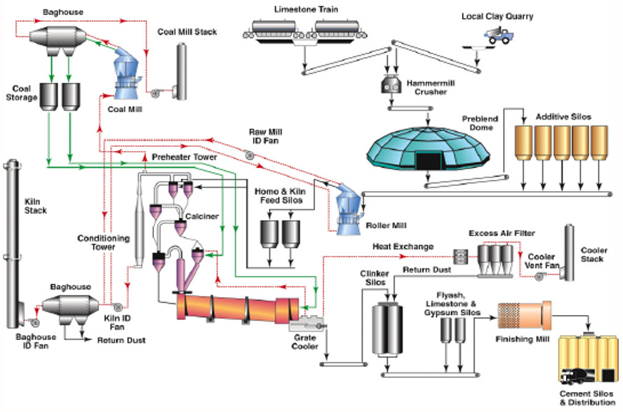 Figure 1: Cement Manufacturing Process (Courtesy of Aixprocess, Barracuda Users Conference 2019) |
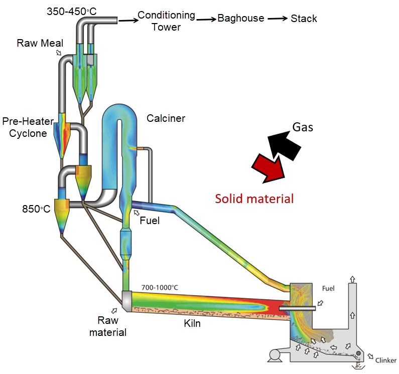 Figure 2: Preheater Tower Flow Diagram (Courtesy of Aixprocess, Barracuda Users Conference 2019)
|
Dating back to the age of the Greek and Roman Empires, cement has remained a staple in industry and society as a critical building material. The process today has come a long way from simply reacting volcanic ash and lime with water. The following process description will relate to Figure 1 and Figure 2. Initially, quarry limestone and clay are crushed down to a processable size in a hammermill crusher. The crushed raw material is now sized appropriately and can be passed through to feed silos where it is stored. Downstream of the silos, the raw material is sent to a preheater tower, which is a series of staged cyclones in which raw materials are fed counter-currently with hot exhaust gas from the Calciner and kiln (Figure 2). As the name suggests, the preheater tower is designed to contact the gas and raw material to raise the particles’ temperature before the raw particles can be sent to the Calciner.
The processes occurring downstream of the preheater tower are highly endothermic, and heating the particles to as high a temperature as possible beforehand will significantly improve process efficiency and reduce the additional energy needed. The now heated particles are calcined, reacted in the kiln, and sent downstream as clinker to be processed further. The conditioning tower falls into place at the fluid exit of the preheater tower after the exhaust gas has contacted the raw material feed at the top cyclone stage. The purpose of the conditioning tower is to cool the exhaust gas significantly to ensure that downstream process equipment is not damaged. After passing through the preheater and the conditioning tower, the cooled gas still needs to be filtered to remove any remaining fines before being vented through a stack, and this usually happens in a Baghouse separator or an Electrostatic Precipitator (ESP). The Baghouse filters are susceptible to changes in operating conditions, such as gas temperature. If the flue gas is fed at higher temperatures than what is rated for the filter bags, then there is a real risk of filter bags degrading much faster than regular maintenance schedules. Frequent filter replacement in a Baghouse is highly undesirable from a process standpoint due to the associated downtime and the high costs associated with the replacement. Hence, the gas must be sufficiently cooled in the conditioning tower before reaching the process equipment further downstream.
Only the top-stage cyclones and the conditioning tower are included in this application model. Heated raw material and exhaust gas from the Calciner and kiln are fed into two cyclone inlets, and the coarser particles are separated, leaving exhaust gas and the unseparated fines to be fed into the conditioning tower. It is assumed that the raw material has transferred heat with the gas, and both species arrive at the cyclone inlets at the same temperature. Upon entering the conditioning tower, water droplets dispersed from eight evenly spaced nozzles are injected, and the mixture of hot gas and particles is cooled. Cooling in the conditioning tower is evaporative, with water droplets being injected, absorbing heat from the exhaust gas and ultimately evaporating completely. Barracuda Virtual Reactor’s (Barracuda Virtual Reactor’s) evaporative modeling capabilities can be utilized to study and optimize the gas cooling in a conditioning tower or any other evaporative cooling applications. The effects of process variables, such as droplet injection rate, location, and the number/spacing of nozzles on gas cooling, can be studied and optimized quickly and efficiently using CFD.
The following application model describes a theoretical conditioning tower where the flue gas is cooled from 450 ºC (842 ºF) to 250 ºC (482 ºF) while evaporating 100% of the water droplets injected in the straight section of the tower. All inputs (process and CAD) used to build the model have been obtained/derived from publicly available sources and prior process knowledge. The model is not intended to represent any industrial-scale conditioning tower in a cement plant and should not be used to make engineering decisions on design or operation. Instead, the model is intended to demonstrate the evaporative gas cooling modeling capabilities of Barracuda Virtual Reactor software to suggest that realistic industrial models of this nature can be developed with confidence using this software.
Model Definition
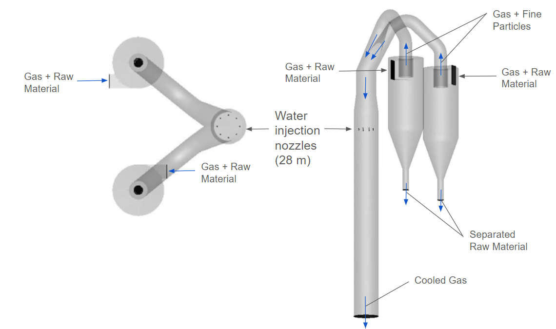
Figure 3: Conditioning Tower Setup
The model setup described for this application is purely based on publicly available information and prior process knowledge. Figure 3 shows the model geometry, 40 m (131.2 ft) tall, 5 m (16.4 ft) in diameter, with two cyclones, both 7.9 m (25.9 ft) tall, 4.3 m (14.1 ft) in diameter, 3.9 m (12.8 ft) in cone height, and a vortex diameter of 1.5 m (4.9 ft). The mesh used for gridding comprises roughly 200,000 cells and was designed to be as coarse as possible while capturing all critical features of the model, specifically the cyclone vortex finders. This cell count and grid resolution are insufficient for industrial-scale simulations, but they provide adequate resolution for demonstrating the gas cooling in the conditioning tower. As mentioned in the introduction, raw material and hot exhaust gas (3.5 mol % O2, 61.5 mol % N2, 28 mol % CO2, and 7 mol % H2O) are fed through the two cyclone inlets, and separated particles are allowed to flow out through the cyclone diplegs. A flow BC is placed at each cyclone inlet, with gas fed at a rate of 37.8 kg/s (300 kpph) and raw material fed at 30.24 kg/s (240 kpph) at a temperature of 450 ºC (842 ºF). Two flow BCs are also placed at each cyclone dipleg, allowing separated particles to exit the cyclone and further aiding in separation. Any fine particles not separated are carried with the gas to the conditioning tower and passed through with injected water droplets. The nozzles themselves are not being modeled, and instead, the effect of the nozzles is being simulated with the use of eight evenly spaced injection BCs. The water is injected with compressed air to aid in dispersion with a total flow rate of 115 USGPM of water (7.24 kg/s) and 400 SCFM (1.72 kg/s) of compressed air. Both are injected at 20 ºC (68 ºF) with an estimated nozzle tip velocity of 205.6 m/s (675 ft/s).
The particle size distributions (PSD) of the kiln feed and the water droplets are based on publicly available literature. A WenYu-Ergun drag model simulates the particle physics and fluid dynamics inside the conditioning tower. The selected material properties for base materials in this model vary with temperature, and all fluids obey the ideal gas equation of state. The evaporation model is enabled for H2O, and the following steps will provide greater detail on this subject and the general setup required to set up the model.
Modeling Instructions:
Simulation Setup:
The application model is based on the “in-built” evaporation model in the Barracuda Virtual Reactor. This model tracks the evaporation and condensation of liquid on particles as a function of both the vapor pressure at the liquid surface and the surrounding vapor partial pressure. An alternative “chemistry-based” approach is also available to model the evaporative process. More information on this approach can be found at this link: https://cpfd-software.com/evaporation-model-for-droplets-and-solid-particle-drying-2024/.
The user is expected to have gone through basic training for Barracuda. Barracuda Virtual Reactor New User Training | CPFD Software (cpfd-software.com)
- Download the provided support files for this application model
- Unzip the file and place it in your working directory.
- Open Barracuda and load the project file CT_mysetup.prj.
- Select File, then Open Project, selecting the specified project folder in your working directory.
The “mysetup” file is loaded with the correct:
- Grid
- Base Materials
- Particle Species
- Initial Conditions
- Boundary Conditions
Not included in the “my-setup” file is the inclusion of an evaporation model for water and heat transfer coefficients for liquid water droplets. The “pre-setup” file containing the completed setup can be run without any additional setup provided as a reference. The following instructions walk through the steps required to complete the model setup using the “my-setup” file.
Global Settings:
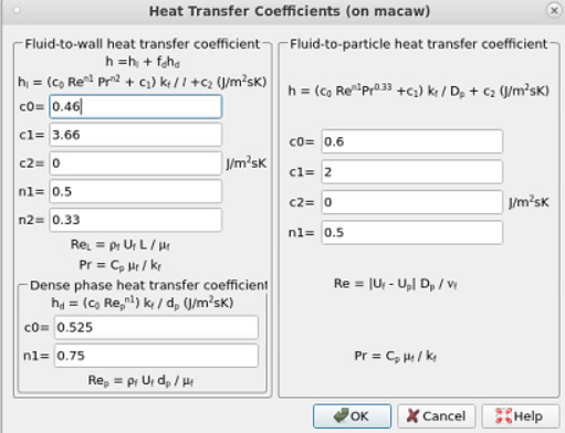
Figure 4: Convective Heat Transfer Coefficient
- Under the Project Tree, select Global Settings and navigate to Heat Transfer Coefficients under Thermal Settings.
- The Heat transfer coefficients for Fluid-to-particle heat transfer are derived from the work of Kunetsov, Strizhak, and Volkov in their paper ” Heat Exchange of an evaporating water droplet in a high-temperature environment.”
\begin{align}
Nu &= \frac{2 + 0.6{Re}^{\frac{1}{2}}{Pr}^{\frac{1}{3}}}{\left(1 – \frac{T_{s}}{T_{a}}\right)^{\frac{T_{s}}{T_{b}}}}
\end{align}
The values from the above equation can be input to determine the convection heat transfer coefficient, as seen in Figure 4. cO is 0.6, c1 is 2, c2 is 0, and n1 is 0.5. Including these values will impact the heat transfer between gas and water droplets and ultimately affect the droplets’ evaporation rate.
Base Materials
Barracuda’s in-built evaporation model can model gas cooling in the conditioning tower. The following instructions describe the model setup.
- Select Base Materials from the project tree and choose H2O (L/V).
- Under Material, toggle the Enable Evaporation Model option to the selected position.
The governing mathematics behind Barracuda’s evaporation model and the corresponding physics of the model are available in the Barracuda Virtual Reactor’s user manual and can be accessed at this link: https://cpfd-software.com/user-manual/base_materials.html#evaporationmodel
Time Controls
- Under Time Step, choose 0.001 seconds.
- Under End Time, choose 70 seconds.
Note that the time step specified is the maximum allowed time step. More aggressive time steps should be avoided in this model to avoid the potential for obtaining inaccurate results. The end time of 70 seconds is roughly 15 seconds after a steady state is reached within the system. The steady state can be established by monitoring dependent variables, such as gas temperature and evaporation rate at different elevations after the water injection.
Visualization Data
- Under the Data Output tab, in Visualization Data, select the following data, as shown in Figure 5.
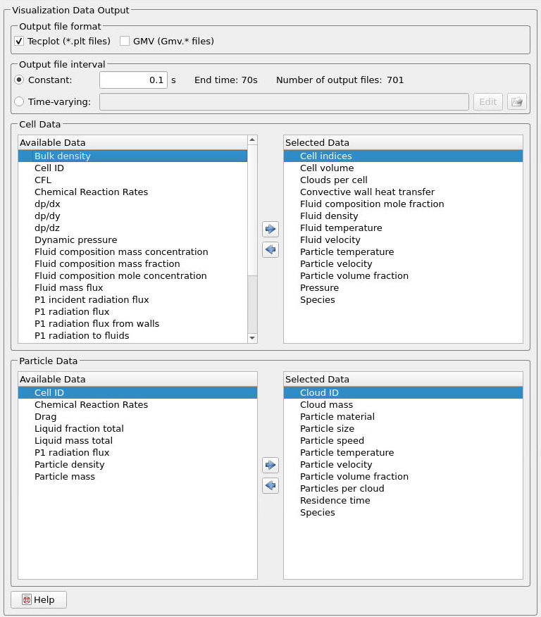
Figure 5: Visualization Data
Run
- Click on Run and then click on Run Solver.
- Select GPU Parallel if you have the required GPU parallel license.
Post Processing with Tecplot
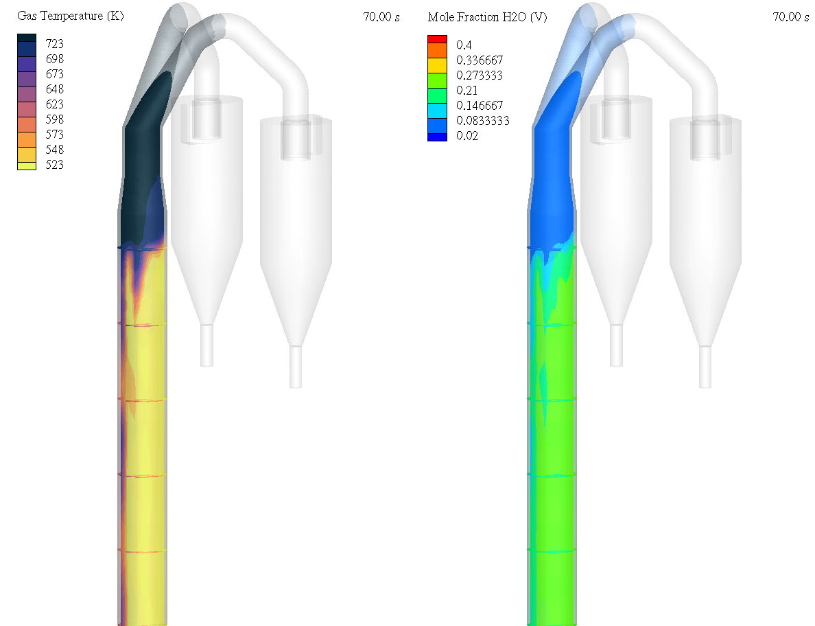
Figure 6: Gas temperature and H2O Mole Fraction Contour Plots.
The user is assumed to have gone through basic Tecplot training. Getting Started With Tecplot For Barracuda® | CPFD Software (cpfd-software.com). A few brief steps for post-processing the results are explained.
- In the Barracuda GUI, click on Post-Run and then click View Results.
- Load in all Barracuda data and Refresh.
- For the left frame, select Z-X under Snap to Orientation View.
- Copy and paste the frames and set Tile Frames from the Quick Macro Panel to 2.
- The following instructions will describe the setup of the top leftmost animation (“Raw Material Temperature” contour).
- Select Particles: Temperature from the Quick Macro Panel.
- Select Slices, and add a slice in group 1 at the origin in the Y plane, ensuring that the Contour is deselected.
- Under other, select Show shade and choose black.
- Under Plot, select Blanking, Value Blanking, and include value blanking when species are not equal to raw material.
- Double-click in the legend and select Levels and Colors.
- Change the color map to CPFD Sand.
- Set Levels from 523 to 723 Kelvin with ten levels.
- Under Legend, change the title and set the number format to an integer.
- The following instructions will describe the setup of the top right-most animation (“Gas Temperature/Droplet Temperature”).
- Select Cells: Fluid Temperature from the Quick Macro Panel.
- Select Slices and add the following two sets of slices:
- Add a slice in group 1 at the origin in the Y plane.
- Add slices in group 2 in the Z plane.
- Select start/end slices, setting the start to 28 (droplet injection) and end at 0 (outlet).
- Select Show intermediate slices and specify 4 for the Number of slices.
- Turn Scatter on and select Particle Temperature.
- Navigate to the value blanking tool as described previously and blank when species is equal to raw material and when X is less than -5.
- Under Zone Style, Effects, Change the Cells Surface Translucency to 80%.
- Under Zone Style, Shade, select Show for the .stl file and include value blanking under Effects.
- Double-click on the Fluid Temperature legend and select Levels and Colors.
- Change the color map to cmocean – oxy.
- Set Levels from 523 to 723 Kelvin with ten levels.
- Under Legend, change the title and set the number format to an integer.
- Do the same for the particle temperature legend, choosing Red/Blue Diverging as the color map.
- The following instructions will describe the setup of the bottom left frame in Figure 6 (“Gas Temperature”).
- Select Contour and de-select Scatter upon opening a new Tecplot results window.
- Selecting the gear icon to the right of the Contour, changing the variable chosen to fluid temperature, changing the color map to cmocean thermal, and ensuring that the color map is reversed.
- In Levels and Color, set levels from 523 to 723 K with nine levels.
- To add the included slices, refer to step 2 of step 6.
- To add the appropriate blanking, blank when X is less than -5.
- Under Zone Style, Shade, select the .stl file and include value blanking under Effects.
- Under Zone Style, Effects, set the cell and .stl file Surface Translucency to 80%.
- The following instructions will describe the setup of the bottom right frame in Figure 6 (Mole Fraction H2O(v)).
- Select Contour and de-select Scatter upon opening a new Tecplot results window.
- Selecting the gear icon to the right of the Contour, change the variable chosen to Fluid domain mole fraction H2O(V), changing the color map to modified rainbow -less green.
- In Levels and Color, set levels from 0.02 to 0.4 with seven levels.
- To add the included slices, refer to step 2 of step 6.
- To add the appropriate blanking, blank when X is less than -5.
- Under Zone Style, Shade, select the .stl file and include value blanking under Effects.
- Under Zone Style, Effects, set the cell and .stl file Surface Translucency to 80%.
Postprocessing: Using PyTecplot
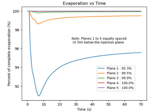 Figure 7: % Evaporation vs Time |
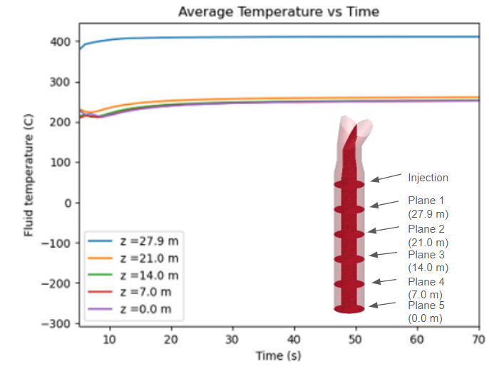 Figure 8: Average Temp vs Time with Plane locations |
The conditioning tower support file includes a Python script that graphs the average temperature and percent evaporation across several flux planes spaced evenly along the tower’s height after water injection (Figure 7 and Figure 8). The data is taken directly from slices in Tecplot, and PyTecplot allows users to use this data in Python scripts. Some brief instructions regarding its use are written below.
- For instructions on how to download Anaconda, refer to the following link: https://cpfd-software.com/installing-the-anaconda-python-distribution/
- Open Jupyter Notebook and open up the jupyter-notebook file from the support directory (python_conditioningTower.ipynb).
- In python_conditioningTower.ipynb:
- Specify the correct file path of the simulation folder.
- Specify the inlet droplet rate as chosen in the injection BC’s (kg/s)
- Specify the Number of planes to be averaged (N).
- To run the code, ensure that PyTecplot connections are enabled. This step must be completed before running the code.
- In Barracuda, navigate to Post-Run, View Results, load all Barracuda data in Tecplot, and select Scripting.
- Select PyTecplot Connections under Scripting and check the box that says Enable Connections.
- Hit Run.
One could alternatively determine the average temperature of the slice solely using Tecplot. Refer to the following link for more information regarding this process: https://cpfd-software.com/tecplot-for-barracuda-calculating-spatial-averages-on-slices/.
Results
Reviewing the graph output using PyTecplot, it is clear that the required reduction in temperature has been met. Particles and gas enter the conditioning tower at 450 ºC (842 ºF) and leave at an approximate average temperature of 250 ºC (482 ºF). All droplets evaporate roughly 14 meters from the tower exit. This has been shown qualitatively in both animations, Figure 6, and quantitatively in Figures 7 and 8. This concludes the description of the Application Model: Cement Plant Conditioning Tower simulation setup process in Barracuda Virtual Reactor.
This concludes the description of the simulation setup process for Application Model: Cement Plant Conditioning Tower in Barracuda Virtual Reactor.