
Introduction
 Foundry cores, depending on geometry, may be difficult to blow uniformly and consistently. Defects are common if the last-to-fill region is not located adjacent to a blow tube. If air cannot exhaust fast enough, back pressure leads to reduced sand particle speeds, creating the potential for soft or miss-filled regions, and resulting in shot-to-shot variability. If sand fronts meet sharply, instead of knitting together, stress cracks may form, either during handling or when encountering hot metal.
Arena-flow’s “Binder coated sand” module simulates the air and sand particle behavior for cold box processes, including sand particle distribution from blow tubes, invests and the blow head.
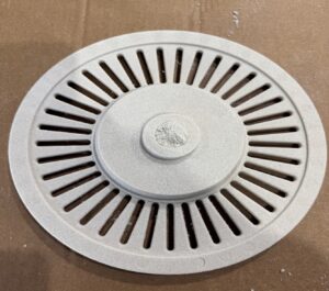
This Application Model demonstrates Arena-flow simulation of a rotor core for a brake disc blown in a single cavity where sand enters the cavity through a single, central blow tube. Application models are sample cases that can be downloaded, run, and customized by CPFD Software’s user community. This model can facility a software demonstration by new or prospective users or serve as a starting point to show basic usage and best practices.
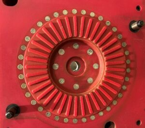
The case is based on blowing a rotor core for an automotive brake disc application, using a single cavity core box made from a red board polymer pattern material. Sand enters the core cavity through a single internal blow tube, while air escapes through discrete vents. This simulation focuses on the individual core behavior assumes an indefinite sand supply from a plenum. Arena-flow can also model the behavior of a finite volume of sand in the magazine, but this added complexity is beyond the scope for this particular application model.
The physical cores, corresponding to this application model, were produced by LaempeReich using 5 bar blow pressure and a 1.5s shoot duration.
Model Definition
Geometry for Arena-flow is defined from the interior tooling surfaces in which the air flows and sand fills. For this model the required geometry consists of the sand plenum, blow tube, and core. All models for Arena-flow must be exported as STL files from 3D modelling software, free of holes, overlaps, intersections, or spikes. High resolution is recommended using a tolerance of 0.01 mm. STL file size is not a concern for an Arena-flow simulation.
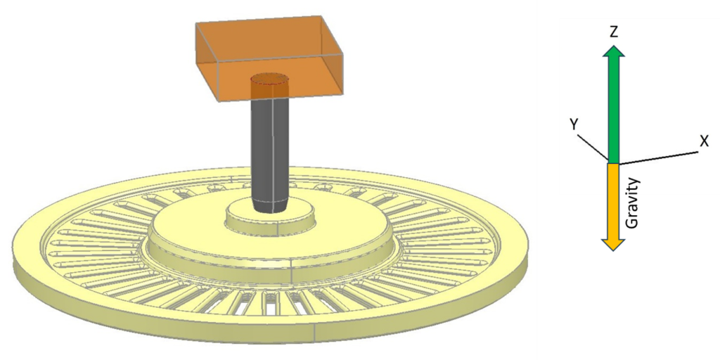
Fig. 1. Model CAD
For this model, the setup consists of a single cavity with a blow tube. Three STL files were created for the plenum, the tube, and the core, although combining models into one STL file is also acceptable. The preferred orientation is for the models to align with the Z axis, with gravity set in the negative Z direction.
A uniform grid is preferred when possible, and a minimum of five cells is recommended with at least one complete cell used in the smallest cross-sectional area of the geometry. For this simulation, a uniform grid of 1,500,000 cells was applied.
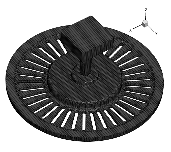
Fig. 2. Computational Grid
Sand type is defined using a predefined particle distribution table, Incast_60.sze. While this application model only uses a single sand type, Arena-flow also permits multiple particle materials and size distributions. Sand location is defined by Particle Volume Fraction and Reference Grid extents. The first sand location uses 0.52, which is the ratio of sand to overall volume in the blow head. Common ranges are 0.52 to 0.55 depending on AFS Grain Fineness Number (GFN). Sand is initialized in the plenum and blow tube, but not in the core, using the (I,J,K) indices of the cells containing the sand. This represents realistic initial conditions for simulation of cold box core blowing and shooting.
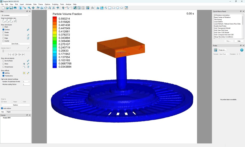
Fig. 3. Initial Sand Conditions
Next, Blow pressure is defined as a pressure plane with a corresponding pressure file, Direction, Area fraction, Particle behavior, and Location. This example assumes a 400,000 Pa blow pressure (gauge pressure) is achieved with a 0.1 second ramp up time. The pressure is then held constant prior to decreasing during an exhaust phase. Direction is selected as the axis that the blow pressure is parallel to. Area fraction is the open area of the pressure plane, and the most common setting is the default value of 1 for unrestricted air flow in the plenum. Particle behavior is set to Feed vol frac for an indefinite sand and particle supply, which is common for a single cavity setup. Location is defined with I, J, K values in the same way as sand locations using the reference grid.
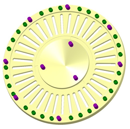
Fig. 4. Drag Vents
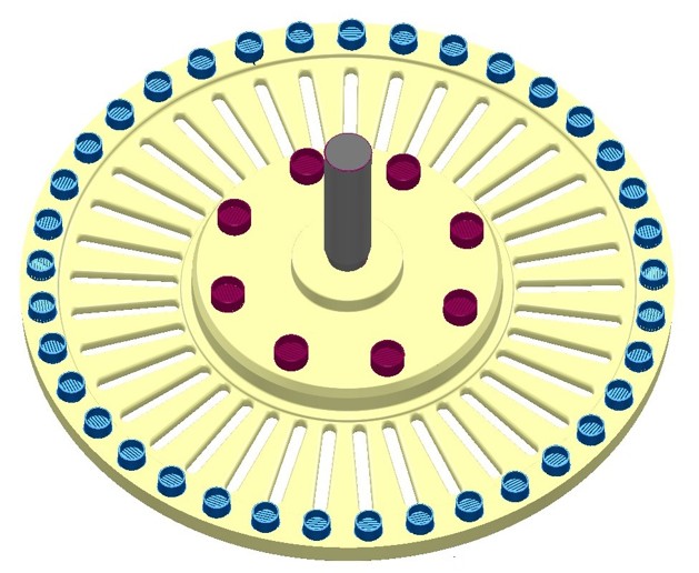
Fig. 5. Cope Vents
Vents are defined using a predefined vent table .tvt file. Predefined cope vents and predefined drag vents are imported, then checked with View Table and View vents under Run. Vent locations are typically exported from CAD software, but can also be created manually or interactively.
Time control, Models, and Data output are set for blowing and filling analysis. End time controls when the solver stops running, which usually corresponds to the core machine setting. Plot interval controls how frequently transient results files (.plt) are written, and for blowing a timestep of 0.01 s is recommended.
Wear settings, Wipe off settings, Flowability settings, and Fill Time settings are left at the advised defaults. The binder percent for predicted resin wipe-off is set to 1.2%, entered as 0.012 in the form. The default Flowability slider position for binder-coated sand between Low and Average is applied for this case. Flowability can be adjusted to account for factors such as binder content, GFN and benchlife.
Default Visualization data settings are generally sufficient, unless the simulation is intended to capture phenomena such as sand segregation by size or density, for example when studying the effect of an additive like iron oxide being added to the sand recipe. Transient data sensor points and Flux planes are created to record localized compaction, pressure, particle speed, and air and particle mass crossing the tube-to-core interface.
Results and Discussion
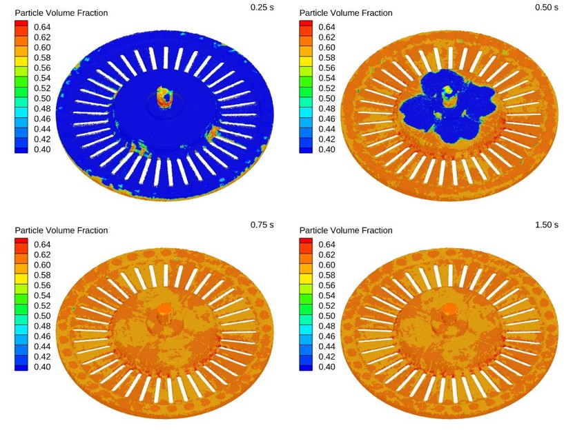
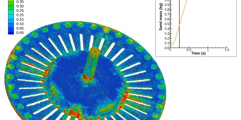
Fig. 6. Particle Volume Fraction, 0.25s to 1.5s
Post-processing is performed using Tecplot for Arena-flow, which is included with an Arena-flow license. Three-dimensional visualization data for this case consists of:
- View filling shows sand particles as pressurized air drags sand into the cavity. Sand particles are colored by Particle volume fraction or sand ratio, meaning the ratio between sand particles and volume of each cell. This view shows how sand flows into the cavity.
- View density shows local in-cell material bulk density, based on the material density of the specified sand particle materials and local compaction. Blue indicates regions of low bulk density, which are potential problem areas.
- View sand speed shows sand particle speed, and is useful when looking at areas with slow moving sand, typically less than 0.2 m/s. Sand moving at less than 0.2 m/s rarely contributes to filling areas that remain soft or miss-filled.
- View pressure shows local in-cell air pressure. Regions in the cavity with limited exhaust, back pressure and stagnant air are of interest. Color gradients changing fast from red to blue are good as they indicate a significant pressure drop, leading to an increase in air velocity and increased drag forces.
- Fill Time gives a quick view of last to fill areas which may be a concern if not located next to a blow tube. Blow tube tracking colors sand by which blow tube it is fed into the cavity. Significant differences in colored area size relating to differences in volumetric input are checked, along with how sand fronts meet and knit together. Sharp fronts could be an issue.
- Wipe off shows predicted areas of resin build up on surfaces by resin volume left on the surface as sand grains move across surfaces before a protective sand layer has formed. Tool wear shows regions prone to high erosion. High wear in blow tubes is normally not a concern unless they wear out fast, since blow tubes are wear parts.
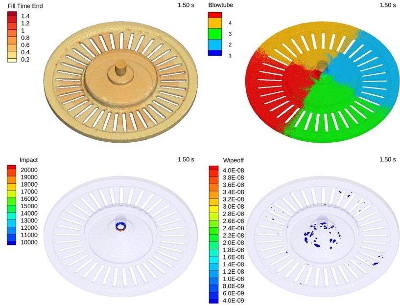
Fig. 7. Fill Time, Blowtube, Impact, and Wipeoff
Flux plane data records air and particle flows crossing a flux plane. Sand mass over time at the tube to core interface can be set up as one flux plane. In this case four flux planes, one for each quadrant, were used to demonstrate the colored sand feature. Flux planes are beneficial when looking at blow tube performance, as mass flows should be as uniform as possible. Graph lines should be as close as possible for the best fill pattern. Steep inclines and sharp turns from incline to horizontal are good, while significant mass differences could indicate a problem with filling.
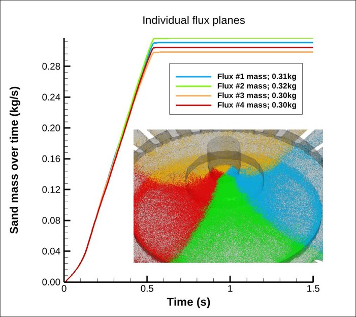
Fig. 8. Flux Planes
Transient data points are useful when looking at localized data like compaction, tracking if there is movement after initial compaction, particle speed and local pressure. In addition to standard outputs, custom results such as air velocity vectors can be generated and displayed using Tecplot for Arena-flow.
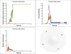
Fig. 9. Transient Data Points
Post-processing of Arena-flow results spanning broad variables including sand motion, speed, core density, and the air flow and pressure profiles, provides a virtual view into core blowing performance prior to the creation of tooling. Arena-flow models, once generated, are easily modified to simulate the impact of variables such as sand types, sand mixtures, additives, blow pressures, tube locations and venting arrangements, directly affecting tooling decisions before cutting metal. Parametric analysis of off-design conditions, such as aged binder and dirty vents, can maximize process robustness.
Modeling Instructions
The user is expected to have already gone through basic Arena-flow training.
- Download the support files provided along with this post.
- Unzip the support file and place it in the working directory set up for this project.
- Open the project file in Arena-flow and verify the grid, setup, and model settings as described in Model Definition.
- Run Solver Setup to generate the initial results file and check the setup, then run the solver to End time.
Post-processing Instructions
To reproduce filling, density, speed, pressure, fill time, and flux views, use the provided layout files from the zipped support file. To load a layout file into Tecplot from the Arena-flow GUI, navigate to Post-Run in the project tree and select either View Results or Launch Tecplot tab, then in Tecplot select File -> Load Layout or File -> Load Arena-flow Data -> Load Layout, navigate to the unzipped support directory and select the .lay file and click on Open.
Set-up from Scratch
This section documents the detailed setup steps for users who want to build the case from scratch rather than starting from the provided project file.
- Grid generation starts by adding the STL files for simulation. Any of the three STL files can be selected in any order, and Open is used to load each file until all are loaded. Shift select cannot be used to open multiple files at the same time. STL Units must then be set, since the grid generator will not run if units are unset and shown in red text color. Double clicking on any selected file in the Geometry STL files box opens the STL information, where a unit that makes sense is selected. In this example units could be either inch or mm, and it is rare for a core to exceed 40 in / 1000 mm. Knowing which casting the core is part of helps with this choice.
- A uniform grid of 1,500,000 cells is applied with Set uniform grid, noting that the uniform grid form does not accept scientific notation. Generate Grid is then used to generate the computational mesh, and the message closes when the grid has been generated. View Output starts Tecplot360 and allows checking the grid for issues using the Grid options in the Quick Macro Panel. As an exercise, three grids using different uniform cell numbers can be generated and checked for grid faults such as spikes in windows, rib connections, shape, and chamfered contact between blow tube, invest and core. The Check_grid.lay layout provides a frame layout for this check.
- Gravity is set with the direction of gravity to Z-. Sand Type is defined by adding a new Particle Species and either using an Excel sheet to create a predefined distribution or browsing for the predefined sand data file Incast_60.sze, which can then be viewed or changed with Edit.
- Sand Location is defined by adding a new location and entering a Particle Volume Fraction of 0.52. The Reference Grid is used with the [ = min and ] = max shortcut keys to position the cursor in the lower and upper corners of the sand magazine and record the I1, J1 and I2, J2 values, with the K1 value noted just below the plenum. After entering a comment and checking the sand location, Apply closes the form. The setup can then be checked under Run with Run Solver Setup and View Sand, before finishing by adding sand in the blow tube.
- Blow Pressure is defined by adding a new pressure plane and either manually creating a pressure file with Edit or continuing with the created blow pressure profile. Direction, Area fraction, and Particle behavior are selected, and Location is applied with I, J, K values in the same way as sand locations using the reference grid. The applied plane is checked under Run with Run Solver Setup and View boundary conditions, where yellow indicates the applied blow pressure.
- Vent definition uses either a new vent table created with New Table or an existing .tvt file selected with Open. The predefined vent tables for cope and drag are continued with for this case, and viewed under Run with Run Solver Setup, Vents, View Table, and View vents.
- Time control is set with End time, a Plot interval of 0.01 s for blowing, and Number of files produced. A running solver is not expected to stop before reaching End time, with changes to End Time possible via Interact and Restart Solver under Run. Models are generally left on, since turning models off would require a rerun. Wear settings are continued without changes to default values, Wipe off binder percent is set to 0.012, the default Flowability slider position between Low and Average is applied, and default Fill settings are generally retained.
- Data output includes Visualization data for additional visual data such as Particle radius, Transient data for individual sensor points defined by Type, location and coordinate values, and Flux planes for 2D planes recording air flow data as air crosses the planes. For flux planes, Enter location by is changed from node to xyz coordinate input before applying, and the flux planes are created as shown in the reference image.
- Run controls include Run Solver setup, which starts the solver and outputs the first result file at T=0.0 s before stopping for Check Setup, Run Solver to continue to End time, Monitor Run to open log files in Tecplot360, Restart Solver to restart from the IC file, and Interact to control the solver. Check Setup outputs are visualized using Tecplot360 with predefined graphics, using only one button before continuing with the Quick Macro panel. Post run analysis under Utilities opens Tecplot360 for post-processing without loading default graphics, views log files such as runtime.log, or opens a terminal in the current project folder, while View results starts Tecplot360, loads the most recent timestep, and displays the selected result.